12 Model Tuning and the Dangers of Overfitting
In order to use a model for prediction, the parameters for that model must be estimated. Some of these parameters can be estimated directly from the training data, but other parameters, called tuning parameters or hyperparameters, must be specified ahead of time and can’t be directly found from training data. These are unknown structural or other kind of values that have significant impact on the model but cannot be directly estimated from the data. This chapter will provide examples of tuning parameters and show how we use tidymodels functions to create and handle tuning parameters. We’ll also demonstrate how poor choices of these values lead to overfitting and introduce several tactics for finding optimal tuning parameters values. Chapters 13 and 14 go into more detail on specific optimization methods for tuning.
12.1 Model Parameters
In ordinary linear regression, there are two parameters \(\beta_0\) and \(\beta_1\) of the model:
\[ y_i = \beta_0 + \beta_1 x_i + \epsilon_i\]
When we have the outcome (\(y\)) and predictor (\(x\)) data, we can estimate the two parameters \(\beta_0\) and \(\beta_1\):
\[\hat \beta_1 = \frac{\sum_i (y_i-\bar{y})(x_i-\bar{x})}{\sum_i(x_i-\bar{x})^2}\]
and
\[\hat \beta_0 = \bar{y}-\hat \beta_1 \bar{x}.\]
We can directly estimate these values from the data for this example model because they are analytically tractable; if we have the data, then we can estimate these model parameters.
There are many situations where a model has parameters that can’t be directly estimated from the data.
For the KNN model, the prediction equation for a new value \(x_0\) is
\[\hat y = \frac{1}{K}\sum_{\ell = 1}^K x_\ell^*\]
where \(K\) is the number of neighbors and the \(x_\ell^*\) are the \(K\) closest values to \(x_0\) in the training set. The model itself is not defined by a model equation; the previous prediction equation instead defines it. This characteristic, along with the possible intractability of the distance measure, makes it impossible to create a set of equations that can be solved for \(K\) (iteratively or otherwise). The number of neighbors has a profound impact on the model; it governs the flexibility of the class boundary. For small values of \(K\), the boundary is very elaborate while for large values, it might be quite smooth.
The number of nearest neighbors is a good example of a tuning parameter or hyperparameter that cannot be directly estimated from the data.
12.2 Tuning Parameters for Different Types of Models
There are many examples of tuning parameters or hyperparameters in different statistical and machine learning models:
Boosting is an ensemble method that combines a series of base models, each of which is created sequentially and depends on the previous models. The number of boosting iterations is an important tuning parameter that usually requires optimization.
In the classic single-layer artificial neural network (a.k.a. the multilayer perceptron), the predictors are combined using two or more hidden units. The hidden units are linear combinations of the predictors that are captured in an activation function (typically a nonlinear function, such as a sigmoid). The hidden units are then connected to the outcome units; one outcome unit is used for regression models, and multiple outcome units are required for classification. The number of hidden units and the type of activation function are important structural tuning parameters.
Modern gradient descent methods are improved by finding the right optimization parameters. Examples of such hyperparameters are learning rates, momentum, and the number of optimization iterations/epochs (Goodfellow, Bengio, and Courville 2016). Neural networks and some ensemble models use gradient descent to estimate the model parameters. While the tuning parameters associated with gradient descent are not structural parameters, they often require tuning.
In some cases, preprocessing techniques require tuning:
In principal component analysis, or its supervised cousin called partial least squares, the predictors are replaced with new, artificial features that have better properties related to collinearity. The number of extracted components can be tuned.
Imputation methods estimate missing predictor values using the complete values of one or more predictors. One effective imputation tool uses \(K\)-nearest neighbors of the complete columns to predict the missing value. The number of neighbors modulates the amount of averaging and can be tuned.
Some classical statistical models also have structural parameters:
In binary regression, the logit link is commonly used (i.e., logistic regression). Other link functions, such as the probit and complementary log-log, are also available (Dobson 1999). This example is described in more detail in the Section 12.3.
Non-Bayesian longitudinal and repeated measures models require a specification for the covariance or correlation structure of the data. Options include compound symmetric (a.k.a. exchangeable), autoregressive, Toeplitz, and others (Littell, Pendergast, and Natarajan 2000).
A counterexample where it is inappropriate to tune a parameter is the prior distribution required for Bayesian analysis. The prior encapsulates the analyst’s belief about the distribution of a quantity before evidence or data are taken into account. For example, in Section 11.4, we used a Bayesian ANOVA model, and we were unclear about what the prior should be for the regression parameters (beyond being a symmetric distribution). We chose a t-distribution with one degree of freedom for the prior since it has heavier tails; this reflects our added uncertainty. Our prior beliefs should not be subject to optimization. Tuning parameters are typically optimized for performance whereas priors should not be tweaked to get “the right results.”
Another (perhaps more debatable) counterexample of a parameter that does not need to be tuned is the number of trees in a random forest or bagging model. This value should instead be chosen to be large enough to ensure numerical stability in the results; tuning it cannot improve performance as long as the value is large enough to produce reliable results. For random forests, this value is typically in the thousands while the number of trees needed for bagging is around 50 to 100.
12.3 What do we Optimize?
How should we evaluate models when we optimize tuning parameters? It depends on the model and the purpose of the model.
For cases where the statistical properties of the tuning parameter are tractable, common statistical properties can be used as the objective function. For example, in the case of binary logistic regression, the link function can be chosen by maximizing the likelihood or information criteria. However, these statistical properties may not align with the results achieved using accuracy-oriented properties. As an example, Friedman (2001) optimized the number of trees in a boosted tree ensemble and found different results when maximizing the likelihood and accuracy:
degrading the likelihood by overfitting actually improves misclassification error rate. Although perhaps counterintuitive, this is not a contradiction; likelihood and error rate measure different aspects of fit quality.
To demonstrate, consider the classification data shown in Figure 12.1 with two predictors, two classes, and a training set of 593 data points.
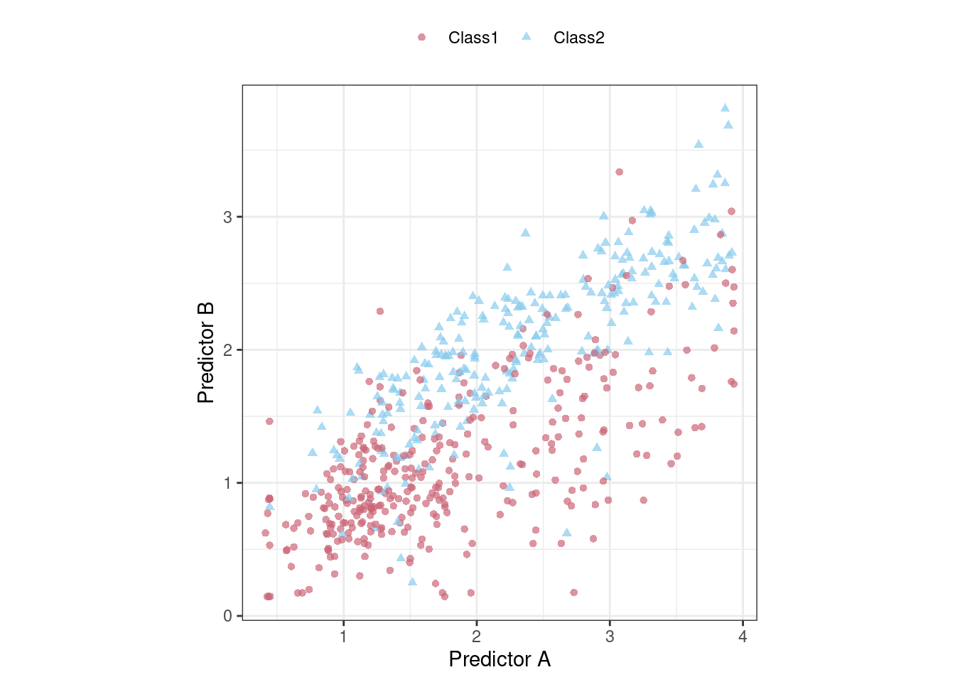
Figure 12.1: An example two-class classification data set with two predictors
We could start by fitting a linear class boundary to these data. The most common method for doing this is to use a generalized linear model in the form of logistic regression. This model relates the log odds of a sample being Class 1 using the logit transformation:
\[ \log\left(\frac{\pi}{1 - \pi}\right) = \beta_0 + \beta_1x_1 + \ldots + \beta_px_p\]
In the context of generalized linear models, the logit function is the link function between the outcome (\(\pi\)) and the predictors. There are other link functions that include the probit model:
\[\Phi^{-1}(\pi) = \beta_0 + \beta_1x_1 + \ldots + \beta_px_p\]
where \(\Phi\) is the cumulative standard normal function, as well as the complementary log-log model:
\[\log(-\log(1-\pi)) = \beta_0 + \beta_1x_1 + \ldots + \beta_px_p\]
Each of these models results in linear class boundaries. Which one should we use? Since, for these data, the number of model parameters does not vary, the statistical approach is to compute the (log) likelihood for each model and determine the model with the largest value. Traditionally, the likelihood is computed using the same data that were used to estimate the parameters, not using approaches like data splitting or resampling from Chapters 5 and 10.
For a data frame training_set, let’s create a function to compute the different models and extract the likelihood statistics for the training set (using broom::glance()):
library(tidymodels)
tidymodels_prefer()

llhood <- function(...) {
  logistic_reg() %>%
    set_engine("glm", ...) %>%
    fit(Class ~ ., data = training_set) %>%
    glance() %>%
    select(logLik)
}

bind_rows(
  llhood(),
  llhood(family = binomial(link = "probit")),
  llhood(family = binomial(link = "cloglog"))
) %>%
  mutate(link = c("logit", "probit", "c-log-log"))  %>%
  arrange(desc(logLik))
#> # A tibble: 3 × 2
#>   logLik link
#>    <dbl> <chr>
#> 1  -258. logit
#> 2  -262. probit
#> 3  -270. c-log-log
According to these results, the logistic model has the best statistical properties.
From the scale of the log-likelihood values, it is difficult to understand if these differences are important or negligible. One way of improving this analysis is to resample the statistics and separate the modeling data from the data used for performance estimation. With this small data set, repeated 10-fold cross-validation is a good choice for resampling. In the yardstick package, the mn_log_loss() function is used to estimate the negative log-likelihood, with our results shown in Figure 12.2.
set.seed(1201)
rs <- vfold_cv(training_set, repeats = 10)

# Return the individual resampled performance estimates:
lloss <- function(...) {
  perf_meas <- metric_set(roc_auc, mn_log_loss)

  logistic_reg() %>%
    set_engine("glm", ...) %>%
    fit_resamples(Class ~ A + B, rs, metrics = perf_meas) %>%
    collect_metrics(summarize = FALSE) %>%
    select(id, id2, .metric, .estimate)
}

resampled_res <-
  bind_rows(
    lloss()                                    %>% mutate(model = "logistic"),
    lloss(family = binomial(link = "probit"))  %>% mutate(model = "probit"),
    lloss(family = binomial(link = "cloglog")) %>% mutate(model = "c-log-log")
  ) %>%
  # Convert log-loss to log-likelihood:
  mutate(.estimate = ifelse(.metric == "mn_log_loss", -.estimate, .estimate)) %>%
  group_by(model, .metric) %>%
  summarize(
    mean = mean(.estimate, na.rm = TRUE),
    std_err = sd(.estimate, na.rm = TRUE) / sqrt(n()),
    .groups = "drop"
  )

resampled_res %>%
  filter(.metric == "mn_log_loss") %>%
  ggplot(aes(x = mean, y = model)) +
  geom_point() +
  geom_errorbar(aes(xmin = mean - 1.64 * std_err, xmax = mean + 1.64 * std_err),
                width = .1) +
  labs(y = NULL, x = "log-likelihood")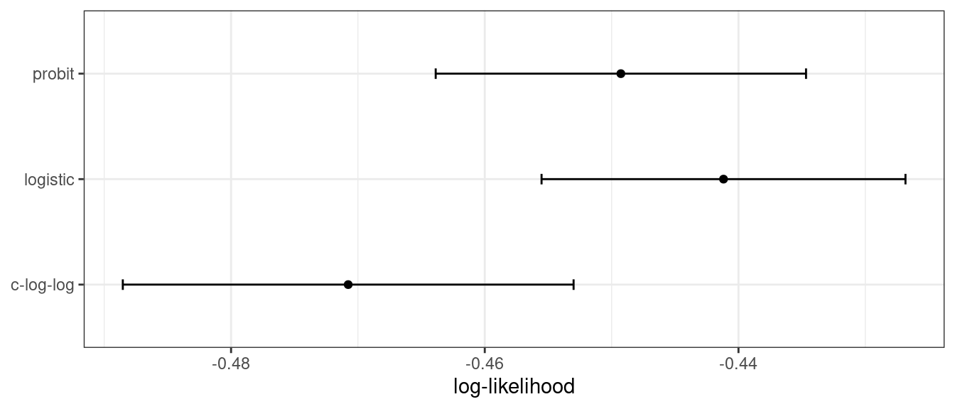
Figure 12.2: Means and approximate 90% confidence intervals for the resampled binomial log-likelihood with three different link functions
The scale of these values is different than the previous values since they are computed on a smaller data set; the value produced by broom::glance() is a sum while yardstick::mn_log_loss() is an average.
These results exhibit evidence that the choice of the link function matters somewhat. Although there is an overlap in the confidence intervals, the logistic model has the best results.
What about a different metric? We also calculated the area under the ROC curve for each resample. These results, which reflect the discriminative ability of the models across numerous probability thresholds, show a lack of difference in Figure 12.3.
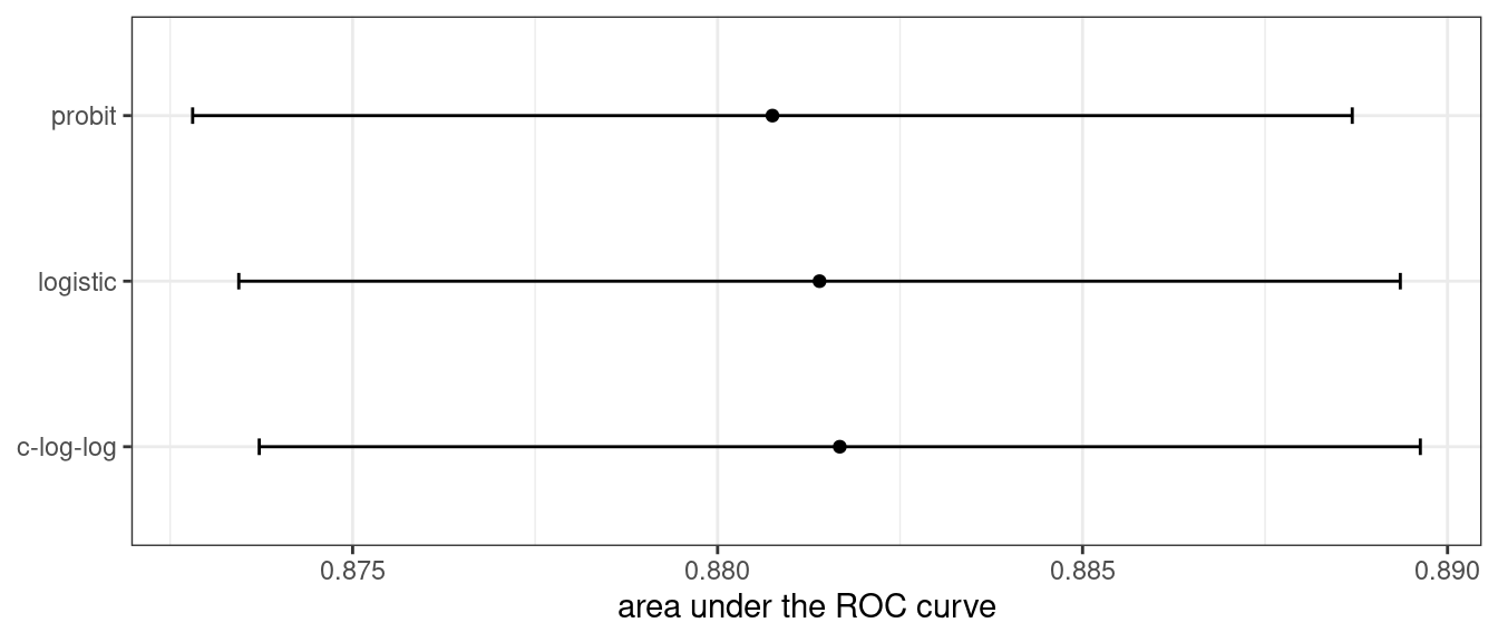
Figure 12.3: Means and approximate 90% confidence intervals for the resampled area under the ROC curve with three different link functions
Given the overlap of the intervals, as well as the scale of the x-axis, any of these options could be used. We see this again when the class boundaries for the three models are overlaid on the test set of 198 data points in Figure 12.4.
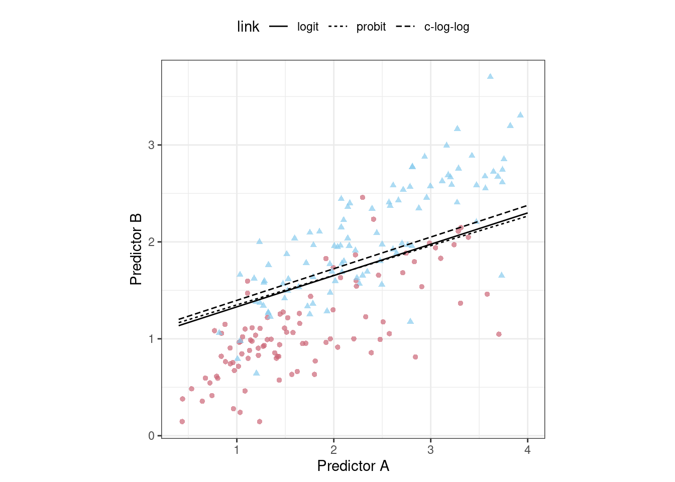
Figure 12.4: The linear class boundary fits for three link functions
This exercise emphasizes that different metrics might lead to different decisions about the choice of tuning parameter values. In this case, one metric indicates the models are somewhat different while another metric shows no difference at all.
Metric optimization is thoroughly discussed by Thomas and Uminsky (2020) who explore several issues, including the gaming of metrics. They warn that:
The unreasonable effectiveness of metric optimization in current AI approaches is a fundamental challenge to the field, and yields an inherent contradiction: solely optimizing metrics leads to far from optimal outcomes.
12.4 The consequences of poor parameter estimates
Many tuning parameters modulate the amount of model complexity. More complexity often implies more malleability in the patterns that a model can emulate. For example, as shown in Section 8.4.3, adding degrees of freedom in a spline function increases the intricacy of the prediction equation. While this is an advantage when the underlying motifs in the data are complex, it can also lead to overinterpretation of chance patterns that would not reproduce in new data. Overfitting is the situation where a model adapts too much to the training data; it performs well for the data used to build the model but poorly for new data.
Since tuning model parameters can increase model complexity, poor choices can lead to overfitting.
Recall the single layer neural network model described in Section 12.2. With a single hidden unit and sigmoidal activation functions, a neural network for classification is, for all intents and purposes, just logistic regression. However, as the number of hidden units increases, so does the complexity of the model. In fact, when the network model uses sigmoidal activation units, Cybenko (1989) showed that the model is a universal function approximator as long as there are enough hidden units.
We fit neural network classification models to the same two-class data from the previous section, varying the number of hidden units. Using the area under the ROC curve as a performance metric, the effectiveness of the model on the training set increases as more hidden units are added. The network model thoroughly and meticulously learns the training set. If the model judges itself on the training set ROC value, it prefers many hidden units so that it can nearly eliminate errors.
Chapters 5 and 10 demonstrated that simply repredicting the training set is a poor approach to model evaluation. Here, the neural network very quickly begins to overinterpret patterns that it sees in the training set. Compare these three example class boundaries (developed with the training set) overlaid on training and test sets in Figure 12.5.
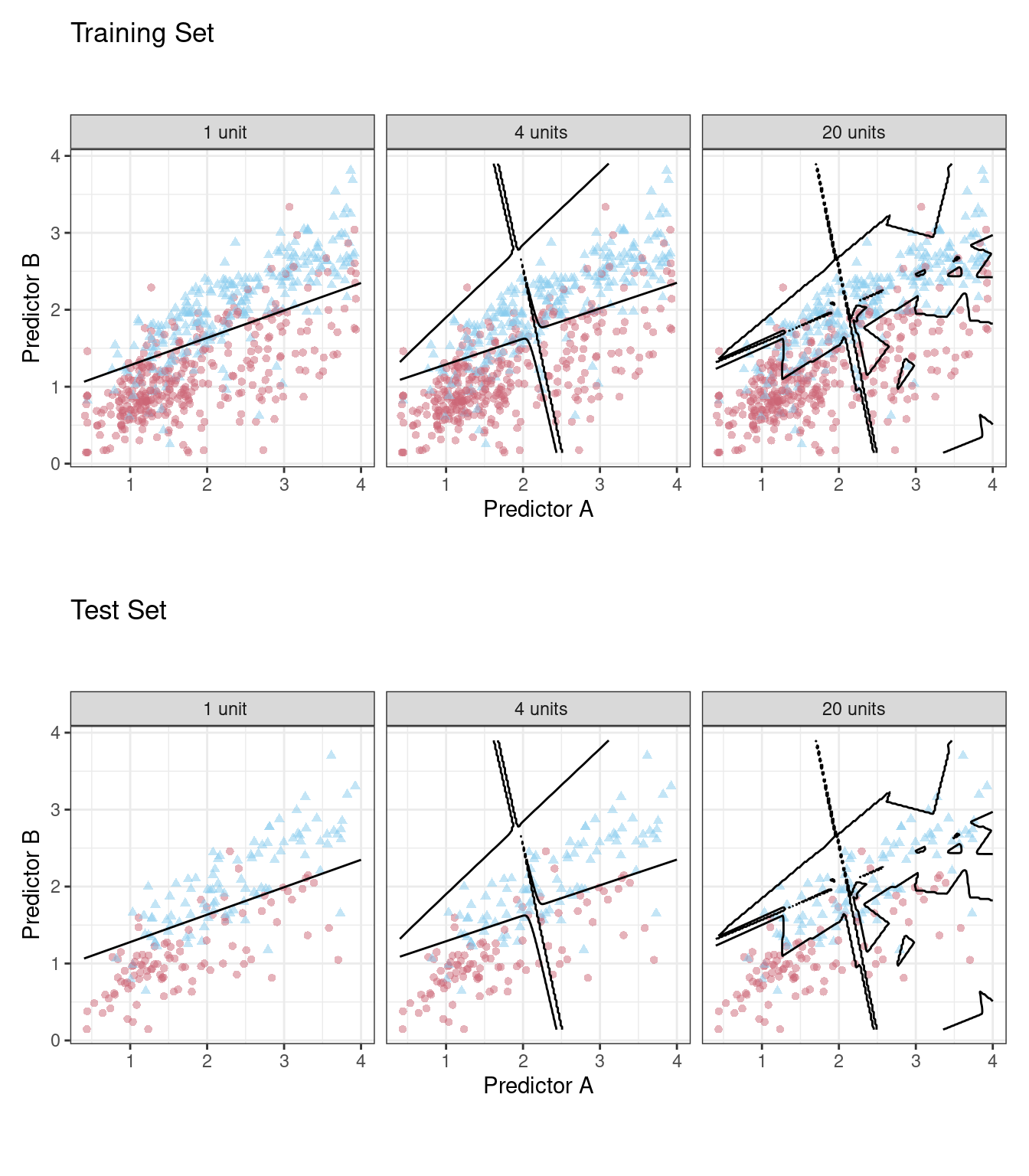
Figure 12.5: Class boundaries for three models with increasing numbers of hidden units. The boundaries are fit on the training set and shown for the training and test sets.
The single unit model does not adapt very flexibly to the data (since it is constrained to be linear). A model with four hidden units begins to show signs of overfitting with an unrealistic boundary for values away from the data mainstream. This is caused by a single data point from the first class in the upper-right corner of the data. By 20 hidden units, the model is beginning to memorize the training set, creating small islands around those data to minimize the resubstitution error rate. These patterns do not repeat in the test set. This last panel is the best illustration of how tuning parameters that control complexity must be modulated so that the model is effective. For a 20-unit model, the training set ROC AUC is 0.944 but the test set value is 0.855.
This occurrence of overfitting is obvious with two predictors that we can plot. However, in general, we must use a quantitative approach for detecting overfitting.
The solution for detecting when a model is overemphasizing the training set is using out-of-sample data.
Rather than using the test set, some form of resampling is required. This could mean an iterative approach (e.g., 10-fold cross-validation) or a single data source (e.g., a validation set).
12.5 Two general strategies for optimization
Tuning parameter optimization usually falls into one of two categories: grid search and iterative search.
Grid search is when we predefine a set of parameter values to evaluate. The main choices involved in grid search are how to make the grid and how many parameter combinations to evaluate. Grid search is often judged as inefficient since the number of grid points required to cover the parameter space can become unmanageable with the curse of dimensionality. There is truth to this concern, but it is most true when the process is not optimized. This is discussed more in Chapter 13.
Iterative search or sequential search is when we sequentially discover new parameter combinations based on previous results. Almost any nonlinear optimization method is appropriate, although some are more efficient than others. In some cases, an initial set of results for one or more parameter combinations is required to start the optimization process. Iterative search is discussed more in Chapter 14.
Figure 12.6 shows two panels that demonstrate these two approaches for a situation with two tuning parameters that range between zero and one. In each, a set of contours shows the true (simulated) relationship between the parameters and the outcome. The optimal results are in the upper-right-hand corners.
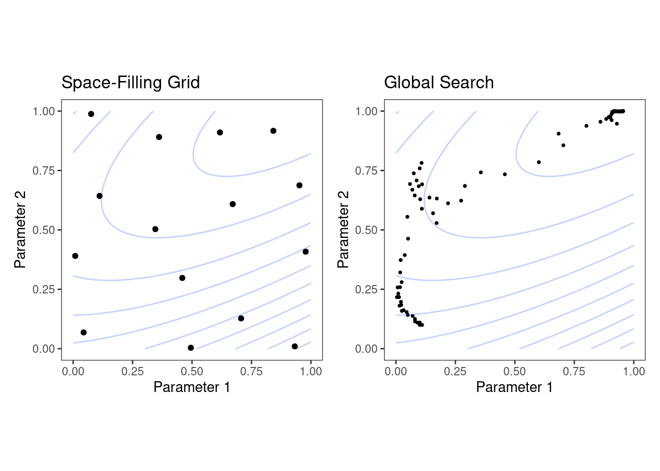
Figure 12.6: Examples of pre-defined grid tuning and an iterative search method. The lines represent contours of a performance metric; it is best in the upper-right-hand side of the plot.
The left-hand panel of Figure 12.6 shows a type of grid called a space-filling design. This is a type of experimental design devised for covering the parameter space such that tuning parameter combinations are not close to one another. The results for this design do not place any points exactly at the truly optimal location. However, one point is in the general vicinity and would probably have performance metric results that are within the noise of the most optimal value.
The right-hand panel of Figure 12.6 illustrates the results of a global search method: the Nelder-Mead simplex method (Olsson and Nelson 1975). The starting point is in the lower-left part of the parameter space. The search meanders across the space until it reaches the optimum location, where it strives to come as close as possible to the numerically best value. This particular search method, while effective, is not known for its efficiency; it requires many function evaluations, especially near the optimal values. Chapter 14 discusses more efficient search algorithms.
Hybrid strategies are also an option and can work well. After an initial grid search, a sequential optimization can start from the best grid combination.
Examples of these strategies are discussed in detail in the next two chapters. Before moving on, let’s learn how to work with tuning parameter objects in tidymodels, using the dials package.
12.6 Tuning Parameters in tidymodels
We’ve already dealt with quite a number of arguments that correspond to tuning parameters for recipe and model specifications in previous chapters. It is possible to tune:
the threshold for combining neighborhoods into an “other” category (with argument name
threshold) discussed in Section 8.4.1the number of degrees of freedom in a natural spline (
deg_free, Section 8.4.3)the number of data points required to execute a split in a tree-based model (
min_n, Section 6.1)the amount of regularization in penalized models (
penalty, Section 6.1)
For parsnip model specifications, there are two kinds of parameter arguments. Main arguments are those that are most often optimized for performance and are available in multiple engines. The main tuning parameters are top-level arguments to the model specification function. For example, the rand_forest() function has main arguments trees, min_n, and mtry since these are most frequently specified or optimized.
A secondary set of tuning parameters are engine specific. These are either infrequently optimized or are specific only to certain engines. Again using random forests as an example, the ranger package contains some arguments that are not used by other packages. One example is gain penalization, which regularizes the predictor selection in the tree induction process. This parameter can help modulate the trade-off between the number of predictors used in the ensemble and performance (Wundervald, Parnell, and Domijan 2020). The name of this argument in ranger() is regularization.factor. To specify a value via a parsnip model specification, it is added as a supplemental argument to set_engine():
rand_forest(trees = 2000, min_n = 10) %>%                   # <- main arguments
  set_engine("ranger", regularization.factor = 0.5)         # <- engine-specific
The main arguments use a harmonized naming system to remove inconsistencies across engines while engine-specific arguments do not.
How can we signal to tidymodels functions which arguments should be optimized? Parameters are marked for tuning by assigning them a value of tune(). For the single layer neural network used in Section 12.4, the number of hidden units is designated for tuning using:
neural_net_spec <-
  mlp(hidden_units = tune()) %>%
  set_mode("regression") %>%
  set_engine("keras")
The tune() function doesn’t execute any particular parameter value; it only returns an expression:
tune()
#> tune()
Embedding this tune() value in an argument will tag the parameter for optimization. The model tuning functions shown in the next two chapters parse the model specification and/or recipe to discover the tagged parameters. These functions can automatically configure and process these parameters since they understand their characteristics (e.g., the range of possible values, etc.).
To enumerate the tuning parameters for an object, use the extract_parameter_set_dials() function:
extract_parameter_set_dials(neural_net_spec)
#> Collection of 1 parameters for tuning
#>
#>    identifier         type    object
#>  hidden_units hidden_units nparam[+]
The results show a value of nparam[+], indicating that the number of hidden units is a numeric parameter.
There is an optional identification argument that associates a name with the parameters. This can come in handy when the same kind of parameter is being tuned in different places. For example, with the Ames housing data from Section 10.6, the recipe encoded both longitude and latitude with spline functions. If we want to tune the two spline functions to potentially have different levels of smoothness, we call step_ns() twice, once for each predictor. To make the parameters identifiable, the identification argument can take any character string:
ames_rec <-
  recipe(Sale_Price ~ Neighborhood + Gr_Liv_Area + Year_Built + Bldg_Type +
           Latitude + Longitude, data = ames_train)  %>%
  step_log(Gr_Liv_Area, base = 10) %>%
  step_other(Neighborhood, threshold = tune()) %>%
  step_dummy(all_nominal_predictors()) %>%
  step_interact( ~ Gr_Liv_Area:starts_with("Bldg_Type_") ) %>%
  step_ns(Longitude, deg_free = tune("longitude df")) %>%
  step_ns(Latitude,  deg_free = tune("latitude df"))

recipes_param <- extract_parameter_set_dials(ames_rec)
recipes_param
#> Collection of 3 parameters for tuning
#>
#>    identifier      type    object
#>     threshold threshold nparam[+]
#>  longitude df  deg_free nparam[+]
#>   latitude df  deg_free nparam[+]
Note that the identifier and type columns are not the same for both of the spline parameters.
When a recipe and model specification are combined using a workflow, both sets of parameters are shown:
wflow_param <-
  workflow() %>%
  add_recipe(ames_rec) %>%
  add_model(neural_net_spec) %>%
  extract_parameter_set_dials()
wflow_param
#> Collection of 4 parameters for tuning
#>
#>    identifier         type    object
#>  hidden_units hidden_units nparam[+]
#>     threshold    threshold nparam[+]
#>  longitude df     deg_free nparam[+]
#>   latitude df     deg_free nparam[+]
Neural networks are exquisitely capable of emulating nonlinear patterns. Adding spline terms to this type of model is unnecessary; we combined this model and recipe for illustration only.
Each tuning parameter argument has a corresponding function in the dials package. In the vast majority of the cases, the function has the same name as the parameter argument:
hidden_units()
#> # Hidden Units (quantitative)
#> Range: [1, 10]
threshold()
#> Threshold (quantitative)
#> Range: [0, 1]
The deg_free parameter is a counterexample; the notion of degrees of freedom comes up in a variety of different contexts. When used with splines, there is a specialized dials function called spline_degree() that is, by default, invoked for splines:
spline_degree()
#> Spline Degrees of Freedom (quantitative)
#> Range: [1, 10]
The dials package also has a convenience function for extracting a particular parameter object:
# identify the parameter using the id value:
wflow_param %>% extract_parameter_dials("threshold")
#> Threshold (quantitative)
#> Range: [0, 0.1]
Inside the parameter set, the range of the parameters can also be updated in place:
extract_parameter_set_dials(ames_rec) %>%
  update(threshold = threshold(c(0.8, 1.0)))
#> Collection of 3 parameters for tuning
#>
#>    identifier      type    object
#>     threshold threshold nparam[+]
#>  longitude df  deg_free nparam[+]
#>   latitude df  deg_free nparam[+]
The parameter sets created by extract_parameter_set_dials() are consumed by the tidymodels tuning functions (when needed). If the defaults for the tuning parameter objects require modification, a modified parameter set is passed to the appropriate tuning function.
Some tuning parameters depend on the dimensions of the data. For example, the number of nearest neighbors must be between one and the number of rows in the data.
In some cases, it is easy to have reasonable defaults for the range of possible values. In other cases, the parameter range is critical and cannot be assumed. The primary tuning parameter for random forest models is the number of predictor columns that are randomly sampled for each split in the tree, usually denoted as mtry(). Without knowing the number of predictors, this parameter range cannot be preconfigured and requires finalization.
rf_spec <-
  rand_forest(mtry = tune()) %>%
  set_engine("ranger", regularization.factor = tune("regularization")) %>%
  set_mode("regression")

rf_param <- extract_parameter_set_dials(rf_spec)
rf_param
#> Collection of 2 parameters for tuning
#>
#>      identifier                  type    object
#>            mtry                  mtry nparam[?]
#>  regularization regularization.factor nparam[+]
#>
#> Model parameters needing finalization:
#>    # Randomly Selected Predictors ('mtry')
#>
#> See `?dials::finalize` or `?dials::update.parameters` for more information.
Complete parameter objects have [+] in their summary; a value of [?] indicates that at least one end of the possible range is missing. There are two methods for handling this. The first is to use update(), to add a range based on what you know about the data dimensions:
rf_param %>%
  update(mtry = mtry(c(1, 70)))
#> Collection of 2 parameters for tuning
#>
#>      identifier                  type    object
#>            mtry                  mtry nparam[+]
#>  regularization regularization.factor nparam[+]
However, this approach might not work if a recipe is attached to a workflow that uses steps that either add or subtract columns. If those steps are not slated for tuning, the finalize() function can execute the recipe once to obtain the dimensions:
pca_rec <-
  recipe(Sale_Price ~ ., data = ames_train) %>%
  # Select the square-footage predictors and extract their PCA components:
  step_normalize(contains("SF")) %>%
  # Select the number of components needed to capture 95% of
  # the variance in the predictors.
  step_pca(contains("SF"), threshold = .95)

updated_param <-
  workflow() %>%
  add_model(rf_spec) %>%
  add_recipe(pca_rec) %>%
  extract_parameter_set_dials() %>%
  finalize(ames_train)
updated_param
#> Collection of 2 parameters for tuning
#>
#>      identifier                  type    object
#>            mtry                  mtry nparam[+]
#>  regularization regularization.factor nparam[+]
updated_param %>% extract_parameter_dials("mtry")
#> # Randomly Selected Predictors (quantitative)
#> Range: [1, 74]
When the recipe is prepared, the finalize() function learns to set the upper range of mtry to 74 predictors.
Additionally, the results of extract_parameter_set_dials() will include engine-specific parameters (if any). They are discovered in the same way as the main arguments and included in the parameter set. The dials package contains parameter functions for all potentially tunable engine-specific parameters:
rf_param
#> Collection of 2 parameters for tuning
#>
#>      identifier                  type    object
#>            mtry                  mtry nparam[?]
#>  regularization regularization.factor nparam[+]
#>
#> Model parameters needing finalization:
#>    # Randomly Selected Predictors ('mtry')
#>
#> See `?dials::finalize` or `?dials::update.parameters` for more information.
regularization_factor()
#> Gain Penalization (quantitative)
#> Range: [0, 1]
Finally, some tuning parameters are best associated with transformations. A good example of this is the penalty parameter associated with many regularized regression models. This parameter is nonnegative and it is common to vary its values in log units. The primary dials parameter object indicates that a transformation is used by default:
penalty()
#> Amount of Regularization (quantitative)
#> Transformer: log-10 [1e-100, Inf]
#> Range (transformed scale): [-10, 0]
This is important to know, especially when altering the range. New range values must be in the transformed units:
# correct method to have penalty values between 0.1 and 1.0
penalty(c(-1, 0)) %>% value_sample(1000) %>% summary()
#>    Min. 1st Qu.  Median    Mean 3rd Qu.    Max.
#>   0.101   0.181   0.327   0.400   0.589   0.999

# incorrect:
penalty(c(0.1, 1.0)) %>% value_sample(1000) %>% summary()
#>    Min. 1st Qu.  Median    Mean 3rd Qu.    Max.
#>    1.26    2.21    3.68    4.26    5.89   10.00
The scale can be changed if desired with the trans argument. You can use natural units but the same range:
penalty(trans = NULL, range = 10^c(-10, 0))
#> Amount of Regularization (quantitative)
#> Range: [1e-10, 1]
12.7 Chapter Summary
This chapter introduced the process of tuning model hyperparameters that cannot be directly estimated from the data. Tuning such parameters can lead to overfitting, often by allowing a model to grow overly complex, so using resampled data sets together with appropriate metrics for evaluation is important. There are two general strategies for determining the right values, grid search and iterative search, which we will explore in depth in the next two chapters. In tidymodels, the tune() function is used to identify parameters for optimization, and functions from the dials package can extract and interact with tuning parameters objects.