21 Inferential Analysis
In Section 1.2, we outlined a taxonomy of models and said that most models can be categorized as descriptive, inferential, and/or predictive.
Most of the chapters in this book have focused on models from the perspective of the accuracy of predicted values, an important quality of models for all purposes but most relevant for predictive models. Inferential models are usually created not only for their predictions, but also to make inferences or judgments about some component of the model, such as a coefficient value or other parameter. These results are often used to answer some (hopefully) pre-defined questions or hypotheses. In predictive models, predictions on hold-out data are used to validate or characterize the quality of the model. Inferential methods focus on validating the probabilistic or structural assumptions that are made prior to fitting the model.
For example, in ordinary linear regression, the common assumption is that the residual values are independent and follow a Gaussian distribution with a constant variance. While you may have scientific or domain knowledge to lend credence to this assumption for your model analysis, the residuals from the fitted model are usually examined to determine if the assumption was a good idea. As a result, the methods for determining if the model’s assumptions have been met are not as simple as looking at holdout predictions, although that can be very useful as well.
We will use p-values in this chapter. However, the tidymodels framework tends to promote confidence intervals over p-values as a method for quantifying the evidence for an alternative hypothesis. As previously shown in Section 11.4, Bayesian methods are often superior to both p-values and confidence intervals in terms of ease of interpretation (but they can be more computationally expensive).
There has been a push in recent years to move away from p-values in favor of other methods (Wasserstein and Lazar 2016). See Volume 73 of The American Statistician for more information and discussion.
In this chapter, we describe how to use tidymodels for fitting and assessing inferential models. In some cases, the tidymodels framework can help users work with the objects produced by their models. In others, it can help assess the quality of a given model.
21.1 Inference for Count Data
To understand how tidymodels packages can be used for inferential modeling, let’s focus on an example with count data. We’ll use biochemistry publication data from the pscl package. These data consist of information on 915 Ph.D. biochemistry graduates and tries to explain factors that impact their academic productivity (measured via number or count of articles published within three years). The predictors include the gender of the graduate, their marital status, the number of children of the graduate that are at least five years old, the prestige of their department, and the number of articles produced by their mentor in the same time period. The data reflect biochemistry doctorates who finished their education between 1956 and 1963. The data are a somewhat biased sample of all of the biochemistry doctorates given during this period (based on completeness of information).
Recall that in Chapter 19 we asked the question “Is our model applicable for predicting a specific data point?” It is very important to define what populations an inferential analysis applies to. For these data, the results would likely apply to biochemistry doctorates given around the time frame that the data were collected. Does it also apply to other chemistry doctorate types (e.g., medicinal chemistry, etc)? These are important questions to address (and document) when conducting inferential analyses.
A plot of the data shown in Figure 21.1 indicates that many graduates did not publish any articles in this time and that the outcome follows a right-skewed distribution:
library(tidymodels)
tidymodels_prefer()

data("bioChemists", package = "pscl")

ggplot(bioChemists, aes(x = art)) +
  geom_histogram(binwidth = 1, color = "white") +
  labs(x = "Number of articles within 3y of graduation")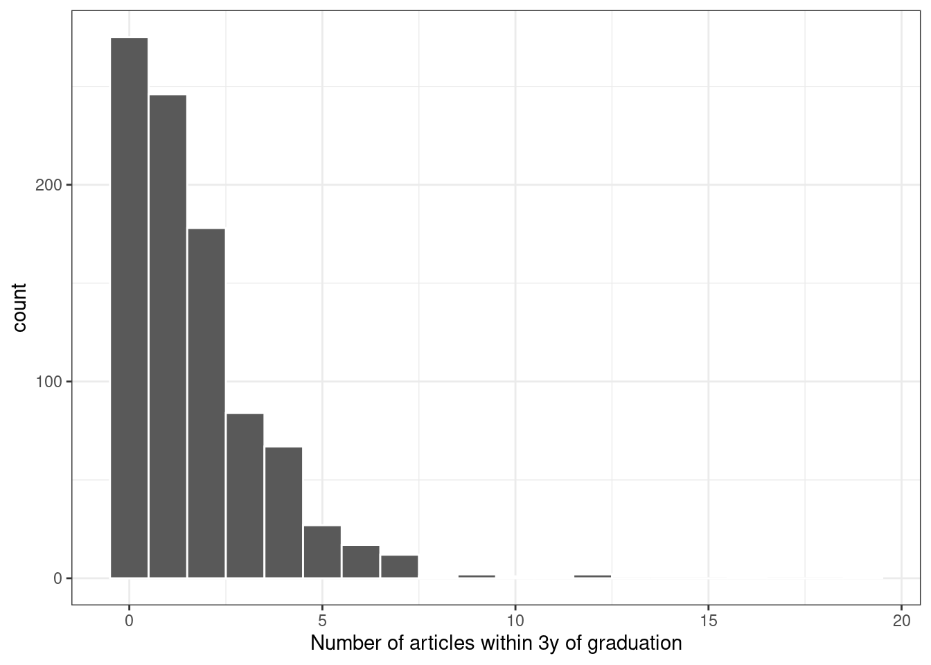
Figure 21.1: Distribution of the number of articles written within 3 years of graduation
Since the outcome data are counts, the most common distribution assumption to make is that the outcome has a Poisson distribution. This chapter will use these data for several types of analyses.
21.2 Comparisons with Two-Sample Tests
We can start with hypothesis testing. The original author’s goal with this data set on biochemistry publication data was to determine if there is a difference in publications between men and women (Long 1992). The data from the study show:
bioChemists %>%
  group_by(fem) %>%
  summarize(counts = sum(art), n = length(art))
#> # A tibble: 2 × 3
#>   fem   counts     n
#>   <fct>  <int> <int>
#> 1 Men      930   494
#> 2 Women    619   421
There were many more publications by men, although there were also more men in the data. The simplest approach to analyzing these data would be to do a two-sample comparison using the poisson.test() function in the stats package. It requires the counts for one or two groups.
For our application, the hypotheses to compare the two sexes are:
\[\begin{align} H_0&: \lambda_m = \lambda_f \notag \\ H_a&: \lambda_m \ne \lambda_f \notag \end{align}\]
where the \(\lambda\) values are the rates of publications (over the same time period).
A basic application of the test is:37
poisson.test(c(930, 619), T = 3)
#>
#>  Comparison of Poisson rates
#>
#> data:  c(930, 619) time base: 3
#> count1 = 930, expected count1 = 774, p-value = 3e-15
#> alternative hypothesis: true rate ratio is not equal to 1
#> 95 percent confidence interval:
#>  1.356 1.666
#> sample estimates:
#> rate ratio
#>      1.502
The function reports a p-value as well as a confidence interval for the ratio of the publication rates. The results indicate that the observed difference is greater than the experiential noise and favors \(H_a\).
One issue with using this function is that the results come back as an htest object. While this type of object has a well-defined structure, it can be difficult to consume for subsequent operations such as reporting or visualizations. The most impactful tool that tidymodels offers for inferential models is the tidy() functions in the broom package. As previously seen, this function makes a well-formed, predictably named tibble from the object. We can tidy() the results of our two-sample comparison test:
poisson.test(c(930, 619)) %>%
  tidy()
#> # A tibble: 1 × 8
#>   estimate statistic  p.value parameter conf.low conf.high method        alternative
#>      <dbl>     <dbl>    <dbl>     <dbl>    <dbl>     <dbl> <chr>         <chr>
#> 1     1.50       930 2.73e-15      774.     1.36      1.67 Comparison o… two.sided
Between the broom and broom.mixed packages, there are tidy() methods for more than 150 models.
While the Poisson distribution is reasonable, we might also want to assess using fewer distributional assumptions. Two methods that might be helpful are the bootstrap and permutation tests (Davison and Hinkley 1997).
The infer package, part of the tidymodels framework, is a powerful and intuitive tool for hypothesis testing (Ismay and Kim 2021). Its syntax is concise and designed for nonstatisticians.
First, we specify() that we will use the difference in the mean number of articles between the sexes and then calculate() the statistic from the data. Recall that the maximum likelihood estimator for the Poisson mean is the sample mean. The hypotheses tested here are the same as the previous test (but are conducted using a different testing procedure).
With infer, we specify the outcome and covariate, then state the statistic of interest:
library(infer)

observed <-
  bioChemists %>%
  specify(art ~ fem) %>%
  calculate(stat = "diff in means", order = c("Men", "Women"))
observed
#> Response: art (numeric)
#> Explanatory: fem (factor)
#> # A tibble: 1 × 1
#>    stat
#>   <dbl>
#> 1 0.412
From here, we compute a confidence interval for this mean by creating the bootstrap distribution via generate(); the same statistic is computed for each resampled version of the data:
set.seed(2101)
bootstrapped <-
  bioChemists %>%
  specify(art ~ fem)  %>%
  generate(reps = 2000, type = "bootstrap") %>%
  calculate(stat = "diff in means", order = c("Men", "Women"))
bootstrapped
#> Response: art (numeric)
#> Explanatory: fem (factor)
#> # A tibble: 2,000 × 2
#>   replicate  stat
#>       <int> <dbl>
#> 1         1 0.467
#> 2         2 0.107
#> 3         3 0.467
#> 4         4 0.308
#> 5         5 0.369
#> 6         6 0.428
#> # ℹ 1,994 more rows
A percentile interval is calculated using:
percentile_ci <- get_ci(bootstrapped)
percentile_ci
#> # A tibble: 1 × 2
#>   lower_ci upper_ci
#>      <dbl>    <dbl>
#> 1    0.158    0.653
The infer package has a high-level API for showing the analysis results, as shown in Figure 21.2.
visualize(bootstrapped) +
    shade_confidence_interval(endpoints = percentile_ci)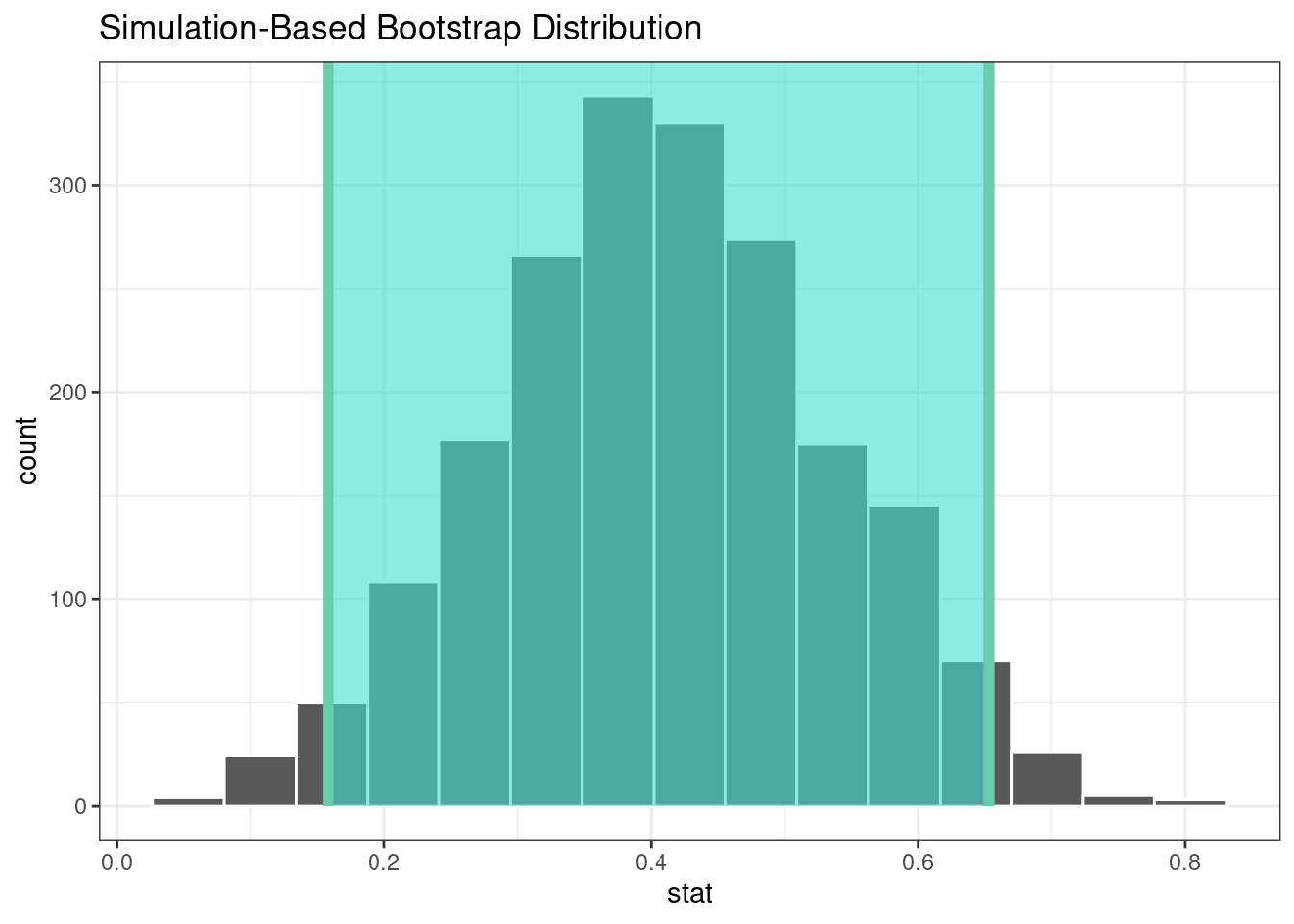
Figure 21.2: The bootstrap distribution of the difference in means. The highlighted region is the confidence interval.
Since the interval visualized in in Figure 21.2 does not include zero, these results indicate that men have published more articles than women.
If we require a p-value, the infer package can compute the value via a permutation test, shown in the following code. The syntax is very similar to the bootstrapping code we used earlier. We add a hypothesize() verb to state the type of assumption to test and the generate() call contains an option to shuffle the data.
set.seed(2102)
permuted <-
  bioChemists %>%
  specify(art ~ fem)  %>%
  hypothesize(null = "independence") %>%
  generate(reps = 2000, type = "permute") %>%
  calculate(stat = "diff in means", order = c("Men", "Women"))
permuted
#> Response: art (numeric)
#> Explanatory: fem (factor)
#> Null Hypothesis: independence
#> # A tibble: 2,000 × 2
#>   replicate     stat
#>       <int>    <dbl>
#> 1         1  0.201
#> 2         2 -0.133
#> 3         3  0.109
#> 4         4 -0.195
#> 5         5 -0.00128
#> 6         6 -0.102
#> # ℹ 1,994 more rows
The following visualization code is also very similar to the bootstrap approach. This code generates Figure 21.3 where the vertical line signifies the observed value:
visualize(permuted) +
    shade_p_value(obs_stat = observed, direction = "two-sided")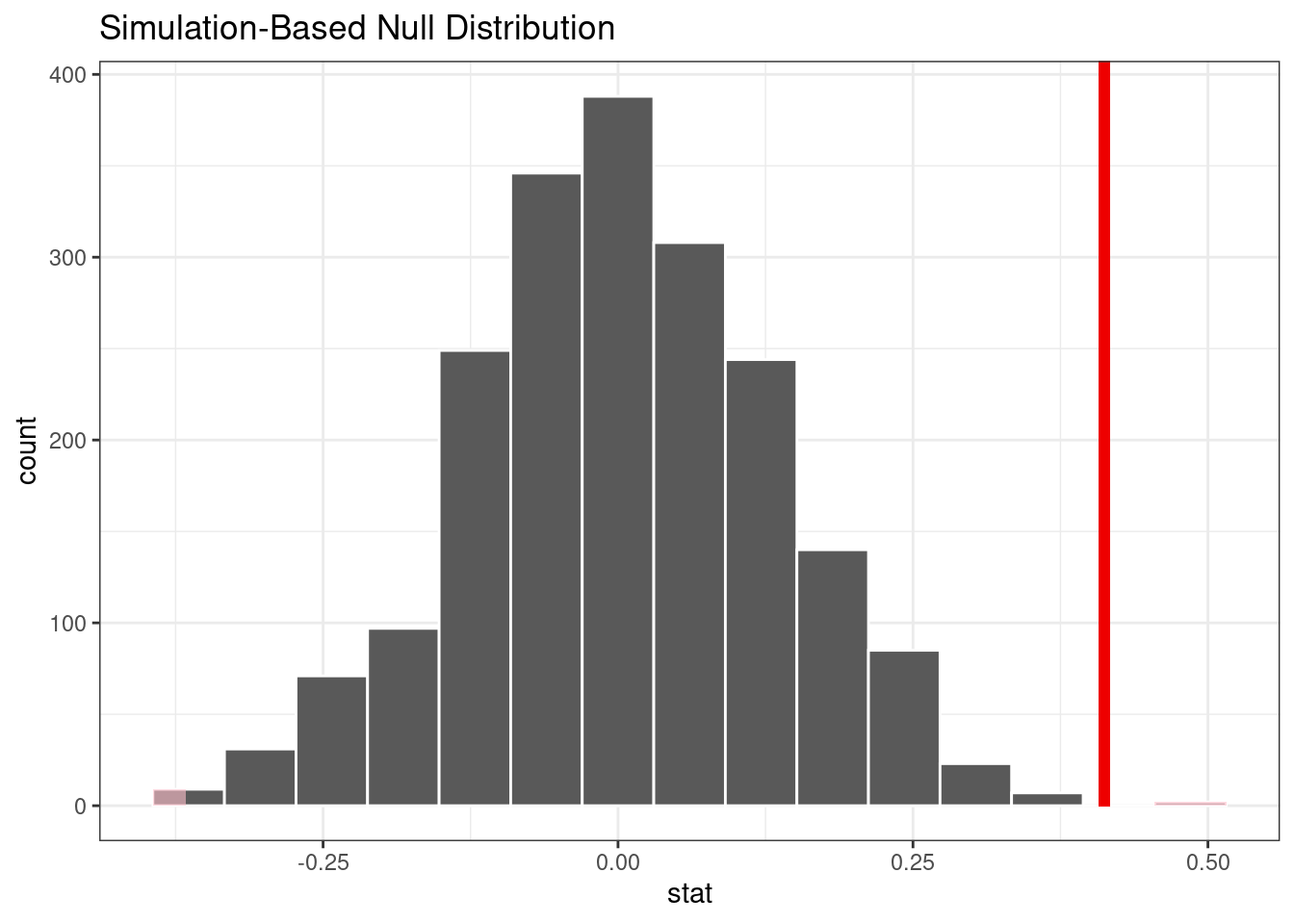
Figure 21.3: Empirical distribution of the test statistic under the null hypothesis. The vertical line indicates the observed test statistic.
The actual p-value is:
permuted %>%
  get_p_value(obs_stat = observed, direction = "two-sided")
#> # A tibble: 1 × 1
#>   p_value
#>     <dbl>
#> 1   0.002
The vertical line representing the null hypothesis in Figure 21.3 is far away from the permutation distribution. This means, if in fact the null hypothesis were true, the likelihood is exceedingly small of observing data at least as extreme as what is at hand.
The two-sample tests shown in this section are probably suboptimal because they do not account for other factors that might explain the observed relationship between publication rate and sex. Let’s move to a more complex model that can consider additional covariates.
21.3 Log-Linear Models
The focus of the rest of this chapter will be on a generalized linear model (Dobson 1999) where we assume the counts follow a Poisson distribution. For this model, the covariates/predictors enter the model in a log-linear fashion:
\[ \log(\lambda) = \beta_0 + \beta_1x_1 + \ldots + \beta_px_p \]
where \(\lambda\) is the expected value of the counts.
Let’s fit a simple model that contains all of the predictor columns. The poissonreg package, a parsnip extension package in tidymodels, will fit this model specification:
library(poissonreg)

# default engine is 'glm'
log_lin_spec <- poisson_reg()

log_lin_fit <-
  log_lin_spec %>%
  fit(art ~ ., data = bioChemists)
log_lin_fit
#> parsnip model object
#>
#>
#> Call:  stats::glm(formula = art ~ ., family = stats::poisson, data = data)
#>
#> Coefficients:
#> (Intercept)     femWomen   marMarried         kid5          phd         ment
#>      0.3046      -0.2246       0.1552      -0.1849       0.0128       0.0255
#>
#> Degrees of Freedom: 914 Total (i.e. Null);  909 Residual
#> Null Deviance:       1820
#> Residual Deviance: 1630  AIC: 3310
The tidy() method succinctly summarizes the coefficients for the model (along with 90% confidence intervals):
tidy(log_lin_fit, conf.int = TRUE, conf.level = 0.90)
#> # A tibble: 6 × 7
#>   term        estimate std.error statistic  p.value conf.low conf.high
#>   <chr>          <dbl>     <dbl>     <dbl>    <dbl>    <dbl>     <dbl>
#> 1 (Intercept)   0.305    0.103       2.96  3.10e- 3   0.134     0.473
#> 2 femWomen     -0.225    0.0546     -4.11  3.92e- 5  -0.315    -0.135
#> 3 marMarried    0.155    0.0614      2.53  1.14e- 2   0.0545    0.256
#> 4 kid5         -0.185    0.0401     -4.61  4.08e- 6  -0.251    -0.119
#> 5 phd           0.0128   0.0264      0.486 6.27e- 1  -0.0305    0.0563
#> 6 ment          0.0255   0.00201    12.7   3.89e-37   0.0222    0.0288
In this output, the p-values correspond to separate hypothesis tests for each parameter:
\[\begin{align} H_0&: \beta_j = 0 \notag \\ H_a&: \beta_j \ne 0 \notag \end{align}\]for each of the model parameters. Looking at these results, phd (the prestige of their department) may not have any relationship with the outcome.
While the Poisson distribution is the routine assumption for data like these, it may be beneficial to conduct a rough check of the model assumptions by fitting the models without using the Poisson likelihood to calculate the confidence intervals. The rsample package has a convenience function to compute bootstrap confidence intervals for lm() and glm() models. We can use this function, while explicitly declaring family = poisson, to compute a large number of model fits. By default, we compute a 90% confidence bootstrap-t interval (percentile intervals are also available):
set.seed(2103)
glm_boot <-
  reg_intervals(art ~ ., data = bioChemists, model_fn = "glm", family = poisson)
glm_boot
#> # A tibble: 5 × 6
#>   term          .lower .estimate  .upper .alpha .method
#>   <chr>          <dbl>     <dbl>   <dbl>  <dbl> <chr>
#> 1 femWomen   -0.358      -0.226  -0.0856   0.05 student-t
#> 2 kid5       -0.298      -0.184  -0.0789   0.05 student-t
#> 3 marMarried  0.000264    0.155   0.317    0.05 student-t
#> 4 ment        0.0182      0.0256  0.0322   0.05 student-t
#> 5 phd        -0.0707      0.0130  0.102    0.05 student-t
When we compare these results (in Figure 21.4) to the purely parametric results from glm(), the bootstrap intervals are somewhat wider. If the data were truly Poisson, these intervals would have more similar widths.
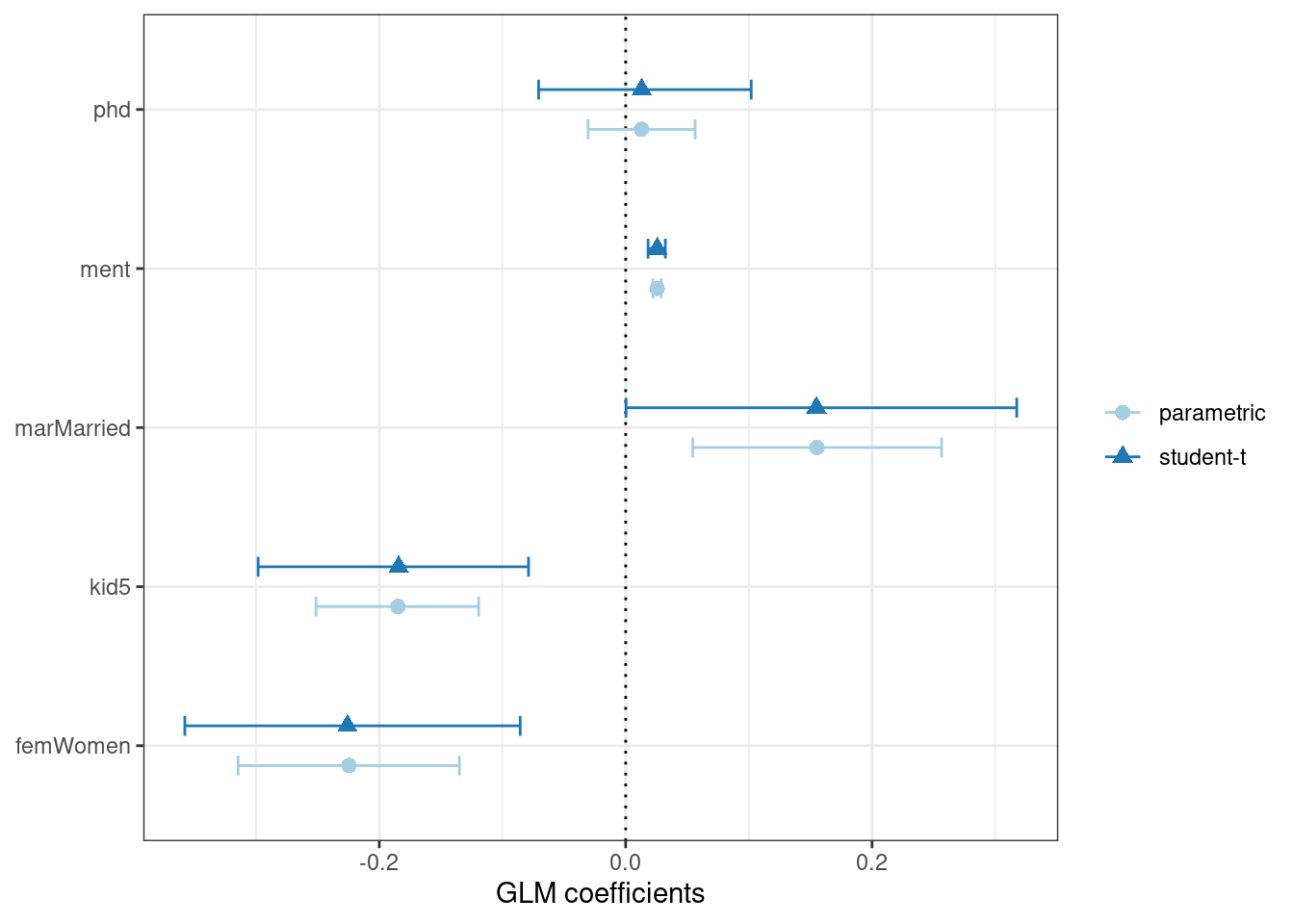
Figure 21.4: Two types of confidence intervals for the Poisson regression model
Determining which predictors to include in the model is a difficult problem. One approach is to conduct likelihood ratio tests (LRT) (McCullagh and Nelder 1989) between nested models. Based on the confidence intervals, we have evidence that a simpler model without phd may be sufficient. Let’s fit a smaller model, then conduct a statistical test:
\[\begin{align} H_0&: \beta_{phd} = 0 \notag \\ H_a&: \beta_{phd} \ne 0 \notag \end{align}\]
This hypothesis was previously tested when we showed the tidied results for log_lin_fit. That particular approach used results from a single model fit via a Wald statistic (i.e., the parameter divided by its standard error). For that approach, the p-value was 0.63. We can tidy the results for the LRT to get the p-value:
log_lin_reduced <-
  log_lin_spec %>%
  fit(art ~ ment + kid5 + fem + mar, data = bioChemists)

anova(
  extract_fit_engine(log_lin_reduced),
  extract_fit_engine(log_lin_fit),
  test = "LRT"
) %>%
  tidy()
#> # A tibble: 2 × 6
#>   term                          df.residual residual.deviance    df deviance p.value
#>   <chr>                               <dbl>             <dbl> <dbl>    <dbl>   <dbl>
#> 1 art ~ ment + kid5 + fem + mar         910             1635.    NA   NA      NA
#> 2 art ~ fem + mar + kid5 + phd…         909             1634.     1    0.236   0.627
The results are the same and, based on these and the confidence interval for this parameter, we’ll exclude phd from further analyses since it does not appear to be associated with the outcome.
21.4 A More Complex Model
We can move into even more complex models within our tidymodels approach. For count data, there are occasions where the number of zero counts is larger than what a simple Poisson distribution would prescribe. A more complex model appropriate for this situation is the zero-inflated Poisson (ZIP) model; see Mullahy (1986), Lambert (1992), and Zeileis, Kleiber, and Jackman (2008). Here, there are two sets of covariates: one for the count data and others that affect the probability (denoted as \(\pi\)) of zeros. The equation for the mean \(\lambda\) is:
\[\lambda = 0 \pi + (1 - \pi) \lambda_{nz}\]
where
\[\begin{align} \log(\lambda_{nz}) &= \beta_0 + \beta_1x_1 + \ldots + \beta_px_p \notag \\ \log\left(\frac{\pi}{1-\pi}\right) &= \gamma_0 + \gamma_1z_1 + \ldots + \gamma_qz_q \notag \end{align}\]and the \(x\) covariates affect the count values while the \(z\) covariates influence the probability of a zero. The two sets of predictors do not need to be mutually exclusive.
We’ll fit a model with a full set of \(z\) covariates:
zero_inflated_spec <- poisson_reg() %>% set_engine("zeroinfl")

zero_inflated_fit <-
  zero_inflated_spec %>%
  fit(art ~ fem + mar + kid5 + ment | fem + mar + kid5 + phd + ment,
      data = bioChemists)

zero_inflated_fit
#> parsnip model object
#>
#>
#> Call:
#> pscl::zeroinfl(formula = art ~ fem + mar + kid5 + ment | fem + mar + kid5 +
#>     phd + ment, data = data)
#>
#> Count model coefficients (poisson with log link):
#> (Intercept)     femWomen   marMarried         kid5         ment
#>       0.621       -0.209        0.105       -0.143        0.018
#>
#> Zero-inflation model coefficients (binomial with logit link):
#> (Intercept)     femWomen   marMarried         kid5          phd         ment
#>     -0.6086       0.1093      -0.3529       0.2195       0.0124      -0.1351
Since the coefficients for this model are also estimated using maximum likelihood, let’s try to use another likelihood ratio test to understand if the new model terms are helpful. We will simultaneously test that:
\[\begin{align} H_0&: \gamma_1 = 0, \gamma_2 = 0, \cdots, \gamma_5 = 0 \notag \\ H_a&: \text{at least one } \gamma \ne 0 \notag \end{align}\]Let’s try ANOVA again:
anova(
  extract_fit_engine(zero_inflated_fit),
  extract_fit_engine(log_lin_reduced),
  test = "LRT"
) %>%
  tidy()
#> Error in UseMethod("anova"): no applicable method for 'anova' applied to an object of class "zeroinfl"
An anova() method isn’t implemented for zeroinfl objects!
An alternative is to use an information criterion statistic, such as the Akaike information criterion (AIC) (Claeskens 2016). This computes the log-likelihood (from the training set) and penalizes that value based on the training set size and the number of model parameters. In R’s parameterization, smaller AIC values are better. In this case, we are not conducting a formal statistical test but estimating the ability of the data to fit the data.
The results indicate that the ZIP model is preferable:
zero_inflated_fit %>% extract_fit_engine() %>% AIC()
#> [1] 3232
log_lin_reduced   %>% extract_fit_engine() %>% AIC()
#> [1] 3312
However, it’s hard to contextualize this pair of single values and assess how different they actually are. To solve this problem, we’ll resample a large number of each of these two models. From these, we can compute the AIC values for each and determine how often the results favor the ZIP model. Basically, we will be characterizing the uncertainty of the AIC statistics to gauge their difference relative to the noise in the data.
We’ll also compute more bootstrap confidence intervals for the parameters in a bit so we specify the apparent = TRUE option when creating the bootstrap samples. This is required for some types of intervals.
First, we create the 4,000 model fits:
zip_form <- art ~ fem + mar + kid5 + ment | fem + mar + kid5 + phd + ment
glm_form <- art ~ fem + mar + kid5 + ment

set.seed(2104)
bootstrap_models <-
  bootstraps(bioChemists, times = 2000, apparent = TRUE) %>%
  mutate(
    glm = map(splits, ~ fit(log_lin_spec,       glm_form, data = analysis(.x))),
    zip = map(splits, ~ fit(zero_inflated_spec, zip_form, data = analysis(.x)))
  )
bootstrap_models
#> # Bootstrap sampling with apparent sample
#> # A tibble: 2,001 × 4
#>   splits            id            glm      zip
#>   <list>            <chr>         <list>   <list>
#> 1 <split [915/355]> Bootstrap0001 <fit[+]> <fit[+]>
#> 2 <split [915/333]> Bootstrap0002 <fit[+]> <fit[+]>
#> 3 <split [915/337]> Bootstrap0003 <fit[+]> <fit[+]>
#> 4 <split [915/344]> Bootstrap0004 <fit[+]> <fit[+]>
#> 5 <split [915/351]> Bootstrap0005 <fit[+]> <fit[+]>
#> 6 <split [915/354]> Bootstrap0006 <fit[+]> <fit[+]>
#> # ℹ 1,995 more rows
Now we can extract the model fits and their corresponding AIC values:
bootstrap_models <-
  bootstrap_models %>%
  mutate(
    glm_aic = map_dbl(glm, ~ extract_fit_engine(.x) %>% AIC()),
    zip_aic = map_dbl(zip, ~ extract_fit_engine(.x) %>% AIC())
  )
mean(bootstrap_models$zip_aic < bootstrap_models$glm_aic)
#> [1] 1
It seems definitive from these results that accounting for the excessive number of zero counts is a good idea.
We could have used fit_resamples() or a workflow set to conduct these computations. In this section, we used mutate() and map() to compute the models to demonstrate how one might use tidymodels tools for models that are not supported by one of the parsnip packages.
Since we have computed the resampled model fits, let’s create bootstrap intervals for the zero probability model coefficients (i.e., the \(\gamma_j\)). We can extract these with the tidy() method and use the type = "zero" option to obtain these estimates:
bootstrap_models <-
  bootstrap_models %>%
  mutate(zero_coefs  = map(zip, ~ tidy(.x, type = "zero")))

# One example:
bootstrap_models$zero_coefs[[1]]
#> # A tibble: 6 × 6
#>   term        type  estimate std.error statistic   p.value
#>   <chr>       <chr>    <dbl>     <dbl>     <dbl>     <dbl>
#> 1 (Intercept) zero   -0.128     0.497     -0.257 0.797
#> 2 femWomen    zero   -0.0764    0.319     -0.240 0.811
#> 3 marMarried  zero   -0.112     0.365     -0.307 0.759
#> 4 kid5        zero    0.270     0.186      1.45  0.147
#> 5 phd         zero   -0.178     0.132     -1.35  0.177
#> 6 ment        zero   -0.123     0.0315    -3.91  0.0000935
It’s a good idea to visualize the bootstrap distributions of the coefficients, as in Figure 21.5.
bootstrap_models %>%
  unnest(zero_coefs) %>%
  ggplot(aes(x = estimate)) +
  geom_histogram(bins = 25, color = "white") +
  facet_wrap(~ term, scales = "free_x") +
  geom_vline(xintercept = 0, lty = 2, color = "gray70")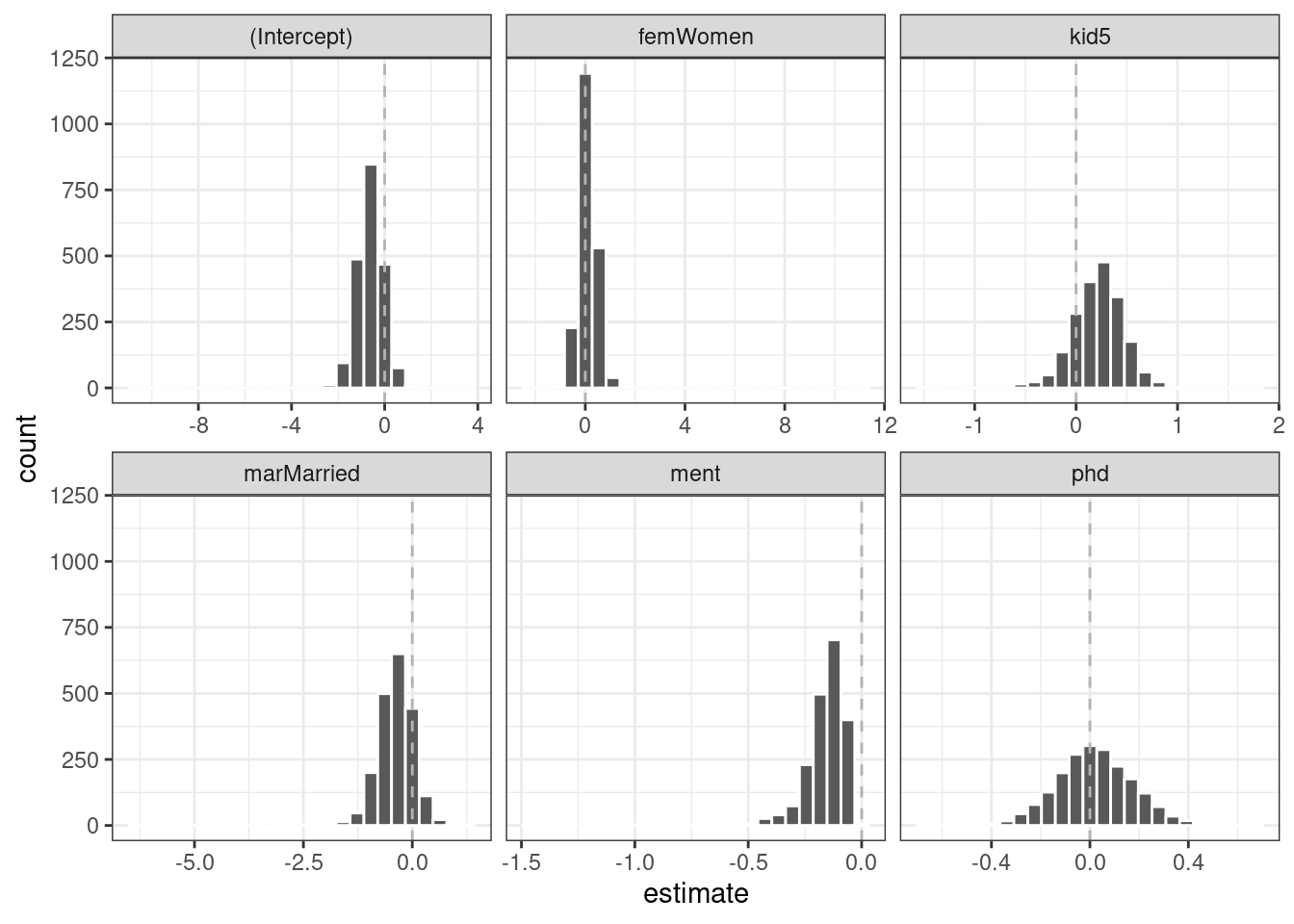
Figure 21.5: Bootstrap distributions of the ZIP model coefficients. The vertical lines indicate the observed estimates.
One of the covariates (ment) that appears to be important has a very skewed distribution. The extra space in some of the facets indicates there are some outliers in the estimates. This might occur when models did not converge; those results probably should be excluded from the resamples. For the results visualized in Figure 21.5, the outliers are due only to extreme parameter estimates; all of the models converged.
The rsample package contains a set of functions named int_*() that compute different types of bootstrap intervals. Since the tidy() method contains standard error estimates, the bootstrap-t intervals can be computed. We’ll also compute the standard percentile intervals. By default, 90% confidence intervals are computed.
bootstrap_models %>% int_pctl(zero_coefs)
#> # A tibble: 6 × 6
#>   term        .lower .estimate  .upper .alpha .method
#>   <chr>        <dbl>     <dbl>   <dbl>  <dbl> <chr>
#> 1 (Intercept) -1.75    -0.621   0.423    0.05 percentile
#> 2 femWomen    -0.521    0.115   0.818    0.05 percentile
#> 3 kid5        -0.327    0.218   0.677    0.05 percentile
#> 4 marMarried  -1.20    -0.381   0.362    0.05 percentile
#> 5 ment        -0.401   -0.162  -0.0513   0.05 percentile
#> 6 phd         -0.276    0.0220  0.327    0.05 percentile
bootstrap_models %>% int_t(zero_coefs)
#> # A tibble: 6 × 6
#>   term        .lower .estimate  .upper .alpha .method
#>   <chr>        <dbl>     <dbl>   <dbl>  <dbl> <chr>
#> 1 (Intercept) -1.61    -0.621   0.321    0.05 student-t
#> 2 femWomen    -0.482    0.115   0.671    0.05 student-t
#> 3 kid5        -0.211    0.218   0.599    0.05 student-t
#> 4 marMarried  -0.988   -0.381   0.290    0.05 student-t
#> 5 ment        -0.324   -0.162  -0.0275   0.05 student-t
#> 6 phd         -0.274    0.0220  0.291    0.05 student-t
From these results, we can get a good idea of which predictor(s) to include in the zero count probability model. It may be sensible to refit a smaller model to assess if the bootstrap distribution for ment is still skewed.
21.5 More Inferential Analysis
This chapter demonstrated just a small subset of what is available for inferential analysis in tidymodels and has focused on resampling and frequentist methods. Arguably, Bayesian analysis is a very effective and often superior approach for inference. A variety of Bayesian models are available via parsnip. Additionally, the multilevelmod package enables users to fit hierarchical Bayesian and non-Bayesian models (e.g., mixed models). The broom.mixed and tidybayes packages are excellent tools for extracting data for plots and summaries. Finally, for data sets with a single hierarchy, such as simple longitudinal or repeated measures data, rsample’s group_vfold_cv() function facilitates straightforward out-of-sample characterizations of model performance.
21.6 Chapter Summary
The tidymodels framework is for more than predictive modeling alone. Packages and functions from tidymodels can be used for hypothesis testing, as well as fitting and assessing inferential models. The tidymodels framework provides support for working with non-tidymodels R models, and can help assess the statistical qualities of your models.
REFERENCES
The
Targument allows us to account for the time when the events (publications) were counted, which was three years for both men and women. There are more men than women in these data, butpoisson.test()has limited functionality so more sophisticated analysis can be used to account for this difference.↩︎