10 Resampling for Evaluating Performance

We have already covered several pieces that must be put together to evaluate the performance of a model. Chapter 9 described statistics for measuring model performance. Chapter 5 introduced the idea of data spending, and we recommended the test set for obtaining an unbiased estimate of performance. However, we usually need to understand the performance of a model or even multiple models before using the test set.

Typically we can’t decide on which final model to use with the test set before first assessing model performance. There is a gap between our need to measure performance reliably and the data splits (training and testing) we have available.

In this chapter, we describe an approach called resampling that can fill this gap. Resampling estimates of performance can generalize to new data in a similar way as estimates from a test set. The next chapter complements this one by demonstrating statistical methods that compare resampling results.

In order to fully appreciate the value of resampling, let’s first take a look the resubstitution approach, which can often fail.

10.1 The Resubstitution Approach

When we measure performance on the same data that we used for training (as opposed to new data or testing data), we say we have resubstituted the data. Let’s again use the Ames housing data to demonstrate these concepts. Section 8.8 summarizes the current state of our Ames analysis. It includes a recipe object named ames_rec, a linear model, and a workflow using that recipe and model called lm_wflow. This workflow was fit on the training set, resulting in lm_fit.

For a comparison to this linear model, we can also fit a different type of model. Random forests are a tree ensemble method that operates by creating a large number of decision trees from slightly different versions of the training set (Breiman 2001a). This collection of trees makes up the ensemble. When predicting a new sample, each ensemble member makes a separate prediction. These are averaged to create the final ensemble prediction for the new data point.

Random forest models are very powerful, and they can emulate the underlying data patterns very closely. While this model can be computationally intensive, it is very low maintenance; very little preprocessing is required (as documented in Appendix A).

Using the same predictor set as the linear model (without the extra preprocessing steps), we can fit a random forest model to the training set via the "ranger" engine (which uses the ranger R package for computation). This model requires no preprocessing, so a simple formula can be used:

rf_model <- 
  rand_forest(trees = 1000) %>% 
  set_engine("ranger") %>% 
  set_mode("regression")

rf_wflow <- 
  workflow() %>% 
  add_formula(
    Sale_Price ~ Neighborhood + Gr_Liv_Area + Year_Built + Bldg_Type + 
      Latitude + Longitude) %>% 
  add_model(rf_model) 

rf_fit <- rf_wflow %>% fit(data = ames_train)

How should we compare the linear and random forest models? For demonstration, we will predict the training set to produce what is known as an apparent metric or resubstitution metric. This function creates predictions and formats the results:

estimate_perf <- function(model, dat) {
  # Capture the names of the `model` and `dat` objects
  cl <- match.call()
  obj_name <- as.character(cl$model)
  data_name <- as.character(cl$dat)
  data_name <- gsub("ames_", "", data_name)
  
  # Estimate these metrics:
  reg_metrics <- metric_set(rmse, rsq)
  
  model %>%
    predict(dat) %>%
    bind_cols(dat %>% select(Sale_Price)) %>%
    reg_metrics(Sale_Price, .pred) %>%
    select(-.estimator) %>%
    mutate(object = obj_name, data = data_name)
}

Both RMSE and \(R^2\) are computed. The resubstitution statistics are:

estimate_perf(rf_fit, ames_train)
#> # A tibble: 2 × 4
#>   .metric .estimate object data 
#>   <chr>       <dbl> <chr>  <chr>
#> 1 rmse       0.0365 rf_fit train
#> 2 rsq        0.960  rf_fit train
estimate_perf(lm_fit, ames_train)
#> # A tibble: 2 × 4
#>   .metric .estimate object data 
#>   <chr>       <dbl> <chr>  <chr>
#> 1 rmse       0.0754 lm_fit train
#> 2 rsq        0.816  lm_fit train

Based on these results, the random forest is much more capable of predicting the sale prices; the RMSE estimate is two-fold better than linear regression. If we needed to choose between these two models for this price prediction problem, we would probably chose the random forest because, on the log scale we are using, its RMSE is about half as large. The next step applies the random forest model to the test set for final verification:

estimate_perf(rf_fit, ames_test)
#> # A tibble: 2 × 4
#>   .metric .estimate object data 
#>   <chr>       <dbl> <chr>  <chr>
#> 1 rmse       0.0704 rf_fit test 
#> 2 rsq        0.852  rf_fit test

The test set RMSE estimate, 0.0704, is much worse than the training set value of 0.0365! Why did this happen?

Many predictive models are capable of learning complex trends from the data. In statistics, these are commonly referred to as low bias models.

In this context, bias is the difference between the true pattern or relationships in data and the types of patterns that the model can emulate. Many black-box machine learning models have low bias, meaning they can reproduce complex relationships. Other models (such as linear/logistic regression, discriminant analysis, and others) are not as adaptable and are considered high bias models.¹⁸

For a low bias model, the high degree of predictive capacity can sometimes result in the model nearly memorizing the training set data. As an obvious example, consider a 1-nearest neighbor model. It will always provide perfect predictions for the training set no matter how well it truly works for other data sets. Random forest models are similar; repredicting the training set will always result in an artificially optimistic estimate of performance.

For both models, Table 10.1 summarizes the RMSE estimate for the training and test sets:

Table 10.1: Performance statistics for training and test sets.

	RMSE Estimates
object	train	test
lm_fit	0.0754	0.0736
rf_fit	0.0365	0.0704

Notice that the linear regression model is consistent between training and testing, because of its limited complexity.¹⁹

The main takeaway from this example is that repredicting the training set will result in an artificially optimistic estimate of performance. It is a bad idea for most models.

If the test set should not be used immediately, and repredicting the training set is a bad idea, what should be done? Resampling methods, such as cross-validation or validation sets, are the solution.

10.2 Resampling Methods

Resampling methods are empirical simulation systems that emulate the process of using some data for modeling and different data for evaluation. Most resampling methods are iterative, meaning that this process is repeated multiple times. The diagram in Figure 10.1 illustrates how resampling methods generally operate.

Figure 10.1: Data splitting scheme from the initial data split to resampling

Resampling is conducted only on the training set, as you see in Figure 10.1. The test set is not involved. For each iteration of resampling, the data are partitioned into two subsamples:

• The model is fit with the analysis set.

• The model is evaluated with the assessment set.

These two subsamples are somewhat analogous to training and test sets. Our language of analysis and assessment avoids confusion with the initial split of the data. These data sets are mutually exclusive. The partitioning scheme used to create the analysis and assessment sets is usually the defining characteristic of the method.

Suppose 20 iterations of resampling are conducted. This means that 20 separate models are fit on the analysis sets, and the corresponding assessment sets produce 20 sets of performance statistics. The final estimate of performance for a model is the average of the 20 replicates of the statistics. This average has very good generalization properties and is far better than the resubstitution estimates.

The next section defines several commonly used resampling methods and discusses their pros and cons.

10.2.1 Cross-validation

Cross-validation is a well established resampling method. While there are a number of variations, the most common cross-validation method is V-fold cross-validation. The data are randomly partitioned into V sets of roughly equal size (called the folds). For illustration, V = 3 is shown in Figure 10.2 for a data set of 30 training set points with random fold allocations. The number inside the symbols is the sample number.

Figure 10.2: V-fold cross-validation randomly assigns data to folds

The color of the symbols in Figure 10.2 represents their randomly assigned folds. Stratified sampling is also an option for assigning folds (previously discussed in Section 5.1).

For three-fold cross-validation, the three iterations of resampling are illustrated in Figure 10.3. For each iteration, one fold is held out for assessment statistics and the remaining folds are substrate for the model. This process continues for each fold so that three models produce three sets of performance statistics.

Figure 10.3: V-fold cross-validation data usage

When V = 3, the analysis sets are 2/3 of the training set and each assessment set is a distinct 1/3. The final resampling estimate of performance averages each of the V replicates.

Using V = 3 is a good choice to illustrate cross-validation, but it is a poor choice in practice because it is too low to generate reliable estimates. In practice, values of V are most often 5 or 10; we generally prefer 10-fold cross-validation as a default because it is large enough for good results in most situations.

What are the effects of changing V? Larger values result in resampling estimates with small bias but substantial variance. Smaller values of V have large bias but low variance. We prefer 10-fold since noise is reduced by replication, but bias is not.²⁰

The primary input is the training set data frame as well as the number of folds (defaulting to 10):

set.seed(1001)
ames_folds <- vfold_cv(ames_train, v = 10)
ames_folds
#> #  10-fold cross-validation 
#> # A tibble: 10 × 2
#>   splits             id    
#>   <list>             <chr> 
#> 1 <split [2107/235]> Fold01
#> 2 <split [2107/235]> Fold02
#> 3 <split [2108/234]> Fold03
#> 4 <split [2108/234]> Fold04
#> 5 <split [2108/234]> Fold05
#> 6 <split [2108/234]> Fold06
#> # ℹ 4 more rows

The column named splits contains the information on how to split the data (similar to the object used to create the initial training/test partition). While each row of splits has an embedded copy of the entire training set, R is smart enough not to make copies of the data in memory.²¹ The print method inside of the tibble shows the frequency of each: [2107/235] indicates that about two thousand samples are in the analysis set and 235 are in that particular assessment set.

These objects also always contain a character column called id that labels the partition.²²

To manually retrieve the partitioned data, the analysis() and assessment() functions return the corresponding data frames:

# For the first fold:
ames_folds$splits[[1]] %>% analysis() %>% dim()
#> [1] 2107   74

The tidymodels packages, such as tune, contain high-level user interfaces so that functions like analysis() are not generally needed for day-to-day work. Section 10.3 demonstrates a function to fit a model over these resamples.

There are a variety of cross-validation variations; we’ll go through the most important ones.

Repeated cross-validation

The most important variation on cross-validation is repeated V-fold cross-validation. Depending on data size or other characteristics, the resampling estimate produced by V-fold cross-validation may be excessively noisy.²³ As with many statistical problems, one way to reduce noise is to gather more data. For cross-validation, this means averaging more than V statistics.

To create R repeats of V-fold cross-validation, the same fold generation process is done R times to generate R collections of V partitions. Now, instead of averaging V statistics, \(V \times R\) statistics produce the final resampling estimate. Due to the Central Limit Theorem, the summary statistics from each model tend toward a normal distribution, as long as we have a lot of data relative to \(V \times R\).

Consider the Ames data. On average, 10-fold cross-validation uses assessment sets that contain roughly 234 properties. If RMSE is the statistic of choice, we can denote that estimate’s standard deviation as \(\sigma\). With simple 10-fold cross-validation, the standard error of the mean RMSE is \(\sigma/\sqrt{10}\). If this is too noisy, repeats reduce the standard error to \(\sigma/\sqrt{10R}\). For 10-fold cross-validation with \(R\) replicates, the plot in Figure 10.4 shows how quickly the standard error²⁴ decreases with replicates.

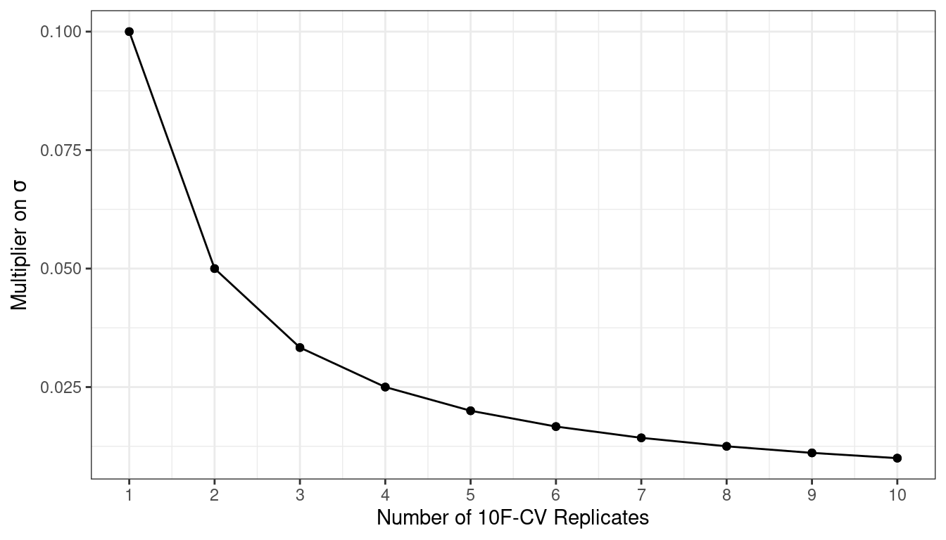
Figure 10.4: Relationship between the relative variance in performance estimates versus the number of cross-validation repeats

Larger numbers of replicates tend to have less impact on the standard error. However, if the baseline value of \(\sigma\) is impractically large, the diminishing returns on replication may still be worth the extra computational costs.

To create repeats, invoke vfold_cv() with an additional argument repeats:

vfold_cv(ames_train, v = 10, repeats = 5)
#> #  10-fold cross-validation repeated 5 times 
#> # A tibble: 50 × 3
#>   splits             id      id2   
#>   <list>             <chr>   <chr> 
#> 1 <split [2107/235]> Repeat1 Fold01
#> 2 <split [2107/235]> Repeat1 Fold02
#> 3 <split [2108/234]> Repeat1 Fold03
#> 4 <split [2108/234]> Repeat1 Fold04
#> 5 <split [2108/234]> Repeat1 Fold05
#> 6 <split [2108/234]> Repeat1 Fold06
#> # ℹ 44 more rows

Leave-one-out cross-validation

One variation of cross-validation is leave-one-out (LOO) cross-validation. If there are \(n\) training set samples, \(n\) models are fit using \(n-1\) rows of the training set. Each model predicts the single excluded data point. At the end of resampling, the \(n\) predictions are pooled to produce a single performance statistic.

Leave-one-out methods are deficient compared to almost any other method. For anything but pathologically small samples, LOO is computationally excessive, and it may not have good statistical properties. Although the rsample package contains a loo_cv() function, these objects are not generally integrated into the broader tidymodels frameworks.

Monte Carlo cross-validation

Another variant of V-fold cross-validation is Monte Carlo cross-validation (MCCV, Xu and Liang (2001)). Like V-fold cross-validation, it allocates a fixed proportion of data to the assessment sets. The difference between MCCV and regular cross-validation is that, for MCCV, this proportion of the data is randomly selected each time. This results in assessment sets that are not mutually exclusive. To create these resampling objects:

mc_cv(ames_train, prop = 9/10, times = 20)
#> # Monte Carlo cross-validation (0.9/0.1) with 20 resamples  
#> # A tibble: 20 × 2
#>   splits             id        
#>   <list>             <chr>     
#> 1 <split [2107/235]> Resample01
#> 2 <split [2107/235]> Resample02
#> 3 <split [2107/235]> Resample03
#> 4 <split [2107/235]> Resample04
#> 5 <split [2107/235]> Resample05
#> 6 <split [2107/235]> Resample06
#> # ℹ 14 more rows

10.2.2 Validation sets

In Section 5.2, we briefly discussed the use of a validation set, a single partition that is set aside to estimate performance separate from the test set. When using a validation set, the initial available data set is split into a training set, a validation set, and a test set (see Figure 10.5).

Figure 10.5: A three-way initial split into training, testing, and validation sets

Validation sets are often used when the original pool of data is very large. In this case, a single large partition may be adequate to characterize model performance without having to do multiple resampling iterations.

With the rsample package, a validation set is like any other resampling object; this type is different only in that it has a single iteration.²⁵ Figure 10.6 shows this scheme.

Figure 10.6: A two-way initial split into training and testing with an additional validation set split on the training set

To build on the code from Section 5.2, the function validation_set() can take the results of initial_validation_split() and convert it to an rset object that is similar to the ones produced by functions such as vfold_cv():

# Previously:

set.seed(52)
# To put 60% into training, 20% in validation, and 20% in testing:
ames_val_split <- initial_validation_split(ames, prop = c(0.6, 0.2))
ames_val_split
#> <Training/Validation/Testing/Total>
#> <1758/586/586/2930>

# Object used for resampling: 
val_set <- validation_set(ames_val_split)
val_set
#> # A tibble: 1 × 2
#>   splits             id        
#>   <list>             <chr>     
#> 1 <split [1758/586]> validation

As you’ll see in Section 10.3, the fit_resamples() function will be used to compute correct estimates of performance using resampling. The val_set object can be used in in this and other functions even though it is a single “resample” of the data.

10.2.3 Bootstrapping

Bootstrap resampling was originally invented as a method for approximating the sampling distribution of statistics whose theoretical properties are intractable (Davison and Hinkley 1997). Using it to estimate model performance is a secondary application of the method.

A bootstrap sample of the training set is a sample that is the same size as the training set but is drawn with replacement. This means that some training set data points are selected multiple times for the analysis set. Each data point has a 63.2% chance of inclusion in the training set at least once. The assessment set contains all of the training set samples that were not selected for the analysis set (on average, with 36.8% of the training set). When bootstrapping, the assessment set is often called the out-of-bag sample.

For a training set of 30 samples, a schematic of three bootstrap samples is shown in Figure10.7.

Figure 10.7: Bootstrapping data usage

Note that the sizes of the assessment sets vary.

Using the rsample package, we can create such bootstrap resamples:

bootstraps(ames_train, times = 5)
#> # Bootstrap sampling 
#> # A tibble: 5 × 2
#>   splits             id        
#>   <list>             <chr>     
#> 1 <split [2342/867]> Bootstrap1
#> 2 <split [2342/869]> Bootstrap2
#> 3 <split [2342/859]> Bootstrap3
#> 4 <split [2342/858]> Bootstrap4
#> 5 <split [2342/873]> Bootstrap5

Bootstrap samples produce performance estimates that have very low variance (unlike cross-validation) but have significant pessimistic bias. This means that, if the true accuracy of a model is 90%, the bootstrap would tend to estimate the value to be less than 90%. The amount of bias cannot be empirically determined with sufficient accuracy. Additionally, the amount of bias changes over the scale of the performance metric. For example, the bias is likely to be different when the accuracy is 90% versus when it is 70%.

The bootstrap is also used inside of many models. For example, the random forest model mentioned earlier contained 1,000 individual decision trees. Each tree was the product of a different bootstrap sample of the training set.

10.2.4 Rolling forecasting origin resampling

When the data have a strong time component, a resampling method should support modeling to estimate seasonal and other temporal trends within the data. A technique that randomly samples values from the training set can disrupt the model’s ability to estimate these patterns.

Rolling forecast origin resampling (Hyndman and Athanasopoulos 2018) provides a method that emulates how time series data is often partitioned in practice, estimating the model with historical data and evaluating it with the most recent data. For this type of resampling, the size of the initial analysis and assessment sets are specified. The first iteration of resampling uses these sizes, starting from the beginning of the series. The second iteration uses the same data sizes but shifts over by a set number of samples.

To illustrate, a training set of fifteen samples was resampled with an analysis size of eight samples and an assessment set size of three. The second iteration discards the first training set sample and both data sets shift forward by one. This configuration results in five resamples, as shown in Figure10.8.

Figure 10.8: Data usage for rolling forecasting origin resampling

Here are two different configurations of this method:

• The analysis set can cumulatively grow (as opposed to remaining the same size). After the first initial analysis set, new samples can accrue without discarding the earlier data.

• The resamples need not increment by one. For example, for large data sets, the incremental block could be a week or month instead of a day.

For a year’s worth of data, suppose that six sets of 30-day blocks define the analysis set. For assessment sets of 30 days with a 29-day skip, we can use the rsample package to specify:

time_slices <- 
  tibble(x = 1:365) %>% 
  rolling_origin(initial = 6 * 30, assess = 30, skip = 29, cumulative = FALSE)

data_range <- function(x) {
  summarize(x, first = min(x), last = max(x))
}

map_dfr(time_slices$splits, ~   analysis(.x) %>% data_range())
#> # A tibble: 6 × 2
#>   first  last
#>   <int> <int>
#> 1     1   180
#> 2    31   210
#> 3    61   240
#> 4    91   270
#> 5   121   300
#> 6   151   330
map_dfr(time_slices$splits, ~ assessment(.x) %>% data_range())
#> # A tibble: 6 × 2
#>   first  last
#>   <int> <int>
#> 1   181   210
#> 2   211   240
#> 3   241   270
#> 4   271   300
#> 5   301   330
#> 6   331   360

10.3 Estimating Performance

Any of the resampling methods discussed in this chapter can be used to evaluate the modeling process (including preprocessing, model fitting, etc). These methods are effective because different groups of data are used to train the model and assess the model. To reiterate, the process to use resampling is:

1. During resampling, the analysis set is used to preprocess the data, apply the preprocessing to itself, and use these processed data to fit the model.

2. The preprocessing statistics produced by the analysis set are applied to the assessment set. The predictions from the assessment set estimate performance on new data.

This sequence repeats for every resample. If there are B resamples, there are B replicates of each of the performance metrics. The final resampling estimate is the average of these B statistics. If B = 1, as with a validation set, the individual statistics represent overall performance.

Let’s reconsider the previous random forest model contained in the rf_wflow object. The fit_resamples() function is analogous to fit(), but instead of having a data argument, fit_resamples() has resamples, which expects an rset object like the ones shown in this chapter. The possible interfaces to the function are:

model_spec %>% fit_resamples(formula,  resamples, ...)
model_spec %>% fit_resamples(recipe,   resamples, ...)
workflow   %>% fit_resamples(          resamples, ...)

There are a number of other optional arguments, such as:

• metrics: A metric set of performance statistics to compute. By default, regression models use RMSE and \(R^2\) while classification models compute the area under the ROC curve and overall accuracy. Note that this choice also defines what predictions are produced during the evaluation of the model. For classification, if only accuracy is requested, class probability estimates are not generated for the assessment set (since they are not needed).

• control: A list created by control_resamples() with various options.

The control arguments include:

• verbose: A logical for printing logging.

• extract: A function for retaining objects from each model iteration (discussed later in this chapter).

• save_pred: A logical for saving the assessment set predictions.

For our example, let’s save the predictions in order to visualize the model fit and residuals:

keep_pred <- control_resamples(save_pred = TRUE, save_workflow = TRUE)

set.seed(1003)
rf_res <- 
  rf_wflow %>% 
  fit_resamples(resamples = ames_folds, control = keep_pred)
rf_res
#> # Resampling results
#> # 10-fold cross-validation 
#> # A tibble: 10 × 5
#>   splits             id     .metrics         .notes           .predictions      
#>   <list>             <chr>  <list>           <list>           <list>            
#> 1 <split [2107/235]> Fold01 <tibble [2 × 4]> <tibble [0 × 3]> <tibble [235 × 4]>
#> 2 <split [2107/235]> Fold02 <tibble [2 × 4]> <tibble [0 × 3]> <tibble [235 × 4]>
#> 3 <split [2108/234]> Fold03 <tibble [2 × 4]> <tibble [0 × 3]> <tibble [234 × 4]>
#> 4 <split [2108/234]> Fold04 <tibble [2 × 4]> <tibble [0 × 3]> <tibble [234 × 4]>
#> 5 <split [2108/234]> Fold05 <tibble [2 × 4]> <tibble [0 × 3]> <tibble [234 × 4]>
#> 6 <split [2108/234]> Fold06 <tibble [2 × 4]> <tibble [0 × 3]> <tibble [234 × 4]>
#> # ℹ 4 more rows

The return value is a tibble similar to the input resamples, along with some extra columns:

• .metrics is a list column of tibbles containing the assessment set performance statistics.

• .notes is another list column of tibbles cataloging any warnings or errors generated during resampling. Note that errors will not stop subsequent execution of resampling.

• .predictions is present when save_pred = TRUE. This list column contains tibbles with the out-of-sample predictions.

While these list columns may look daunting, they can be easily reconfigured using tidyr or with convenience functions that tidymodels provides. For example, to return the performance metrics in a more usable format:

collect_metrics(rf_res)
#> # A tibble: 2 × 6
#>   .metric .estimator   mean     n std_err .config             
#>   <chr>   <chr>       <dbl> <int>   <dbl> <chr>               
#> 1 rmse    standard   0.0721    10 0.00305 Preprocessor1_Model1
#> 2 rsq     standard   0.831     10 0.0108  Preprocessor1_Model1

These are the resampling estimates averaged over the individual replicates. To get the metrics for each resample, use the option summarize = FALSE.

Notice how much more realistic the performance estimates are than the resubstitution estimates from Section 10.1!

To obtain the assessment set predictions:

assess_res <- collect_predictions(rf_res)
assess_res
#> # A tibble: 2,342 × 5
#>   id     .pred  .row Sale_Price .config             
#>   <chr>  <dbl> <int>      <dbl> <chr>               
#> 1 Fold01  5.10    10       5.09 Preprocessor1_Model1
#> 2 Fold01  4.92    27       4.90 Preprocessor1_Model1
#> 3 Fold01  5.21    47       5.08 Preprocessor1_Model1
#> 4 Fold01  5.13    52       5.10 Preprocessor1_Model1
#> 5 Fold01  5.13    59       5.10 Preprocessor1_Model1
#> 6 Fold01  5.13    63       5.11 Preprocessor1_Model1
#> # ℹ 2,336 more rows

The prediction column names follow the conventions discussed for parsnip models in Chapter 6, for consistency and ease of use. The observed outcome column always uses the original column name from the source data. The .row column is an integer that matches the row of the original training set so that these results can be properly arranged and joined with the original data.

For some resampling methods, such as the bootstrap or repeated cross-validation, there will be multiple predictions per row of the original training set. To obtain summarized values (averages of the replicate predictions) use collect_predictions(object, summarize = TRUE).

Since this analysis used 10-fold cross-validation, there is one unique prediction for each training set sample. These data can generate helpful plots of the model to understand where it potentially failed. For example, Figure 10.9 compares the observed and held-out predicted values (analogous to Figure 9.2):

assess_res %>% 
  ggplot(aes(x = Sale_Price, y = .pred)) + 
  geom_point(alpha = .15) +
  geom_abline(color = "red") + 
  coord_obs_pred() + 
  ylab("Predicted")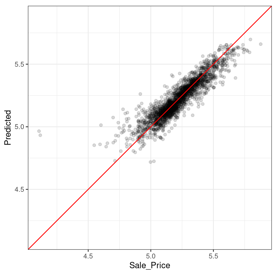

Figure 10.9: Out-of-sample observed versus predicted values for an Ames regression model, using log-10 units on both axes

There are two houses in the training set with a low observed sale price that are significantly overpredicted by the model. Which houses are these? Let’s find out from the assess_res result:

over_predicted <- 
  assess_res %>% 
  mutate(residual = Sale_Price - .pred) %>% 
  arrange(desc(abs(residual))) %>% 
  slice(1:2)
over_predicted
#> # A tibble: 2 × 6
#>   id     .pred  .row Sale_Price .config              residual
#>   <chr>  <dbl> <int>      <dbl> <chr>                   <dbl>
#> 1 Fold09  4.97    32       4.11 Preprocessor1_Model1   -0.858
#> 2 Fold08  4.93   317       4.12 Preprocessor1_Model1   -0.815

ames_train %>% 
  slice(over_predicted$.row) %>% 
  select(Gr_Liv_Area, Neighborhood, Year_Built, Bedroom_AbvGr, Full_Bath)
#> # A tibble: 2 × 5
#>   Gr_Liv_Area Neighborhood           Year_Built Bedroom_AbvGr Full_Bath
#>         <int> <fct>                       <int>         <int>     <int>
#> 1         832 Old_Town                     1923             2         1
#> 2         733 Iowa_DOT_and_Rail_Road       1952             2         1

Identifying examples like these with especially poor performance can help us follow up and investigate why these specific predictions are so poor.

Let’s move back to the homes overall. How can we use a validation set instead of cross-validation? From our previous rsample object:

val_res <- rf_wflow %>% fit_resamples(resamples = val_set)
#> Warning in `[.tbl_df`(x, is.finite(x <- as.numeric(x))): NAs introduced by coercion
val_res
#> # Resampling results
#> #  
#> # A tibble: 1 × 4
#>   splits             id         .metrics         .notes          
#>   <list>             <chr>      <list>           <list>          
#> 1 <split [1758/586]> validation <tibble [2 × 4]> <tibble [0 × 3]>

collect_metrics(val_res)
#> # A tibble: 2 × 6
#>   .metric .estimator   mean     n std_err .config             
#>   <chr>   <chr>       <dbl> <int>   <dbl> <chr>               
#> 1 rmse    standard   0.0728     1      NA Preprocessor1_Model1
#> 2 rsq     standard   0.822      1      NA Preprocessor1_Model1

These results are also much closer to the test set results than the resubstitution estimates of performance.

In these analyses, the resampling results are very close to the test set results. The two types of estimates tend to be well correlated. However, this could be from random chance. A seed value of 55 fixed the random numbers before creating the resamples. Try changing this value and re-running the analyses to investigate whether the resampled estimates match the test set results as well.

10.4 Parallel Processing

The models created during resampling are independent of one another. Computations of this kind are sometimes called embarrassingly parallel; each model could be fit simultaneously without issues.²⁶ The tune package uses the foreach package to facilitate parallel computations. These computations could be split across processors on the same computer or across different computers, depending on the chosen technology.

For computations conducted on a single computer, the number of possible worker processes is determined by the parallel package:

# The number of physical cores in the hardware:
parallel::detectCores(logical = FALSE)
#> [1] 2

# The number of possible independent processes that can 
# be simultaneously used:  
parallel::detectCores(logical = TRUE)
#> [1] 2

The difference between these two values is related to the computer’s processor. For example, most Intel processors use hyperthreading, which creates two virtual cores for each physical core. While these extra resources can improve performance, most of the speed-ups produced by parallel processing occur when processing uses fewer than the number of physical cores.

For fit_resamples() and other functions in tune, parallel processing occurs when the user registers a parallel backend package. These R packages define how to execute parallel processing. On Unix and macOS operating systems, one method of splitting computations is by forking threads. To enable this, load the doMC package and register the number of parallel cores with foreach:

# Unix and macOS only
library(doMC)
registerDoMC(cores = 2)

# Now run fit_resamples()...

This instructs fit_resamples() to run half of the computations on each of two cores. To reset the computations to sequential processing:

registerDoSEQ()

Alternatively, a different approach to parallelizing computations uses network sockets. The doParallel package enables this method (usable by all operating systems):

# All operating systems
library(doParallel)

# Create a cluster object and then register: 
cl <- makePSOCKcluster(2)
registerDoParallel(cl)

# Now run fit_resamples()`...

stopCluster(cl)

Another R package that facilitates parallel processing is the future package. Like foreach, it provides a framework for parallelism. This package is used in conjunction with foreach via the doFuture package.

The R packages with parallel backends for foreach start with the prefix "do".

Parallel processing with the tune package tends to provide linear speed-ups for the first few cores. This means that, with two cores, the computations are twice as fast. Depending on the data and model type, the linear speed-up deteriorates after four to five cores. Using more cores will still reduce the time it takes to complete the task; there are just diminishing returns for the additional cores.

Let’s wrap up with one final note about parallelism. For each of these technologies, the memory requirements multiply for each additional core used. For example, if the current data set is 2 GB in memory and three cores are used, the total memory requirement is 8 GB (2 for each worker process plus the original). Using too many cores might cause the computations (and the computer) to slow considerably.

10.5 Saving the Resampled Objects

The models created during resampling are not retained. These models are trained for the purpose of evaluating performance, and we typically do not need them after we have computed performance statistics. If a particular modeling approach does turn out to be the best option for our data set, then the best choice is to fit again to the whole training set so the model parameters can be estimated with more data.

While these models created during resampling are not preserved, there is a method for keeping them or some of their components. The extract option of control_resamples() specifies a function that takes a single argument; we’ll use x. When executed, x results in a fitted workflow object, regardless of whether you provided fit_resamples() with a workflow. Recall that the workflows package has functions that can pull the different components of the objects (e.g., the model, recipe, etc.).

Let’s fit a linear regression model using the recipe we developed in Chapter 8:

ames_rec <- 
  recipe(Sale_Price ~ Neighborhood + Gr_Liv_Area + Year_Built + Bldg_Type + 
           Latitude + Longitude, data = ames_train) %>%
  step_other(Neighborhood, threshold = 0.01) %>% 
  step_dummy(all_nominal_predictors()) %>% 
  step_interact( ~ Gr_Liv_Area:starts_with("Bldg_Type_") ) %>% 
  step_ns(Latitude, Longitude, deg_free = 20)

lm_wflow <-  
  workflow() %>% 
  add_recipe(ames_rec) %>% 
  add_model(linear_reg() %>% set_engine("lm")) 

lm_fit <- lm_wflow %>% fit(data = ames_train)

# Select the recipe: 
extract_recipe(lm_fit, estimated = TRUE)
#> 
#> ── Recipe ───────────────────────────────────────────────────────────────────────────
#> 
#> ── Inputs
#> Number of variables by role
#> outcome:   1
#> predictor: 6
#> 
#> ── Training information
#> Training data contained 2342 data points and no incomplete rows.
#> 
#> ── Operations
#> • Collapsing factor levels for: Neighborhood | Trained
#> • Dummy variables from: Neighborhood, Bldg_Type | Trained
#> • Interactions with: Gr_Liv_Area:(Bldg_Type_TwoFmCon + Bldg_Type_Duplex +
#>   Bldg_Type_Twnhs + Bldg_Type_TwnhsE) | Trained
#> • Natural splines on: Latitude, Longitude | Trained

We can save the linear model coefficients for a fitted model object from a workflow:

get_model <- function(x) {
  extract_fit_parsnip(x) %>% tidy()
}

# Test it using: 
# get_model(lm_fit)

Now let’s apply this function to the ten resampled fits. The results of the extraction function is wrapped in a list object and returned in a tibble:

ctrl <- control_resamples(extract = get_model)

lm_res <- lm_wflow %>%  fit_resamples(resamples = ames_folds, control = ctrl)
lm_res
#> # Resampling results
#> # 10-fold cross-validation 
#> # A tibble: 10 × 5
#>   splits             id     .metrics         .notes           .extracts       
#>   <list>             <chr>  <list>           <list>           <list>          
#> 1 <split [2107/235]> Fold01 <tibble [2 × 4]> <tibble [0 × 3]> <tibble [1 × 2]>
#> 2 <split [2107/235]> Fold02 <tibble [2 × 4]> <tibble [0 × 3]> <tibble [1 × 2]>
#> 3 <split [2108/234]> Fold03 <tibble [2 × 4]> <tibble [0 × 3]> <tibble [1 × 2]>
#> 4 <split [2108/234]> Fold04 <tibble [2 × 4]> <tibble [0 × 3]> <tibble [1 × 2]>
#> 5 <split [2108/234]> Fold05 <tibble [2 × 4]> <tibble [0 × 3]> <tibble [1 × 2]>
#> 6 <split [2108/234]> Fold06 <tibble [2 × 4]> <tibble [0 × 3]> <tibble [1 × 2]>
#> # ℹ 4 more rows

Now there is a .extracts column with nested tibbles. What do these contain? Let’s find out by subsetting.

lm_res$.extracts[[1]]
#> # A tibble: 1 × 2
#>   .extracts         .config             
#>   <list>            <chr>               
#> 1 <tibble [73 × 5]> Preprocessor1_Model1

# To get the results
lm_res$.extracts[[1]][[1]]
#> [[1]]
#> # A tibble: 73 × 5
#>   term                        estimate  std.error statistic   p.value
#>   <chr>                          <dbl>      <dbl>     <dbl>     <dbl>
#> 1 (Intercept)                 1.48     0.320         4.62   4.11e-  6
#> 2 Gr_Liv_Area                 0.000158 0.00000476   33.2    9.72e-194
#> 3 Year_Built                  0.00180  0.000149     12.1    1.57e- 32
#> 4 Neighborhood_College_Creek -0.00163  0.0373       -0.0438 9.65e-  1
#> 5 Neighborhood_Old_Town      -0.0757   0.0138       -5.47   4.92e-  8
#> 6 Neighborhood_Edwards       -0.109    0.0310       -3.53   4.21e-  4
#> # ℹ 67 more rows

This might appear to be a convoluted method for saving the model results. However, extract is flexible and does not assume that the user will only save a single tibble per resample. For example, the tidy() method might be run on the recipe as well as the model. In this case, a list of two tibbles will be returned.

For our more simple example, all of the results can be flattened and collected using:

all_coef <- map_dfr(lm_res$.extracts, ~ .x[[1]][[1]])
# Show the replicates for a single predictor:
filter(all_coef, term == "Year_Built")
#> # A tibble: 10 × 5
#>   term       estimate std.error statistic  p.value
#>   <chr>         <dbl>     <dbl>     <dbl>    <dbl>
#> 1 Year_Built  0.00180  0.000149      12.1 1.57e-32
#> 2 Year_Built  0.00180  0.000151      12.0 6.45e-32
#> 3 Year_Built  0.00185  0.000150      12.3 1.00e-33
#> 4 Year_Built  0.00183  0.000147      12.5 1.90e-34
#> 5 Year_Built  0.00184  0.000150      12.2 2.47e-33
#> 6 Year_Built  0.00180  0.000150      12.0 3.35e-32
#> # ℹ 4 more rows

Chapters 13 and 14 discuss a suite of functions for tuning models. Their interfaces are similar to fit_resamples() and many of the features described here apply to those functions.

10.6 Chapter Summary

This chapter describes one of the fundamental tools of data analysis, the ability to measure the performance and variation in model results. Resampling enables us to determine how well the model works without using the test set.

An important function from the tune package, called fit_resamples(), was introduced. The interface for this function is also used in future chapters that describe model tuning tools.

The data analysis code, so far, for the Ames data is:

library(tidymodels)
data(ames)
ames <- mutate(ames, Sale_Price = log10(Sale_Price))

set.seed(502)
ames_split <- initial_split(ames, prop = 0.80, strata = Sale_Price)
ames_train <- training(ames_split)
ames_test  <-  testing(ames_split)

ames_rec <- 
  recipe(Sale_Price ~ Neighborhood + Gr_Liv_Area + Year_Built + Bldg_Type + 
           Latitude + Longitude, data = ames_train) %>%
  step_log(Gr_Liv_Area, base = 10) %>% 
  step_other(Neighborhood, threshold = 0.01) %>% 
  step_dummy(all_nominal_predictors()) %>% 
  step_interact( ~ Gr_Liv_Area:starts_with("Bldg_Type_") ) %>% 
  step_ns(Latitude, Longitude, deg_free = 20)

lm_model <- linear_reg() %>% set_engine("lm")

lm_wflow <- 
  workflow() %>% 
  add_model(lm_model) %>% 
  add_recipe(ames_rec)

lm_fit <- fit(lm_wflow, ames_train)

rf_model <- 
  rand_forest(trees = 1000) %>% 
  set_engine("ranger") %>% 
  set_mode("regression")

rf_wflow <- 
  workflow() %>% 
  add_formula(
    Sale_Price ~ Neighborhood + Gr_Liv_Area + Year_Built + Bldg_Type + 
      Latitude + Longitude) %>% 
  add_model(rf_model) 

set.seed(1001)
ames_folds <- vfold_cv(ames_train, v = 10)

keep_pred <- control_resamples(save_pred = TRUE, save_workflow = TRUE)

set.seed(1003)
rf_res <- rf_wflow %>% fit_resamples(resamples = ames_folds, control = keep_pred)

REFERENCES

———. 2001a. “Random Forests.” Machine Learning 45 (1): 5–32.

Davison, A, and D Hinkley. 1997. Bootstrap Methods and Their Application. Vol. 1. Cambridge university press.

Hyndman, R, and G Athanasopoulos. 2018. Forecasting: Principles and Practice. OTexts.

———. 2020. Feature Engineering and Selection: A Practical Approach for Predictive Models. CRC Press.

Schmidberger, M, M Morgan, D Eddelbuettel, H Yu, L Tierney, and U Mansmann. 2009. “State of the Art in Parallel Computing with R.” Journal of Statistical Software 31 (1): 1–27. https://www.jstatsoft.org/v031/i01.

Xu, Q, and Y Liang. 2001. “Monte Carlo Cross Validation.” Chemometrics and Intelligent Laboratory Systems 56 (1): 1–11.

---

18. See Section 1.2.5 of M. Kuhn and Johnson (2020) for a discussion: https://bookdown.org/max/FES/important-concepts.html#model-bias-and-variance↩︎

19. It is possible for a linear model to nearly memorize the training set, like the random forest model did. In the ames_rec object, change the number of spline terms for longitude and latitude to a large number (say 1,000). This would produce a model fit with a very small resubstitution RMSE and a test set RMSE that is much larger.↩︎

20. See Section 3.4 of M. Kuhn and Johnson (2020) for a longer description of the results of changing V: https://bookdown.org/max/FES/resampling.html↩︎

21. To see this for yourself, try executing lobstr::obj_size(ames_folds) and lobstr::obj_size(ames_train). The size of the resample object is much less than ten times the size of the original data.↩︎

22. Some resampling methods require multiple id fields.↩︎

23. For more details, see Section 3.4.6 of M. Kuhn and Johnson (2020): https://bookdown.org/max/FES/resampling.html#resample-var-bias.↩︎

24. These are approximate standard errors. As will be discussed in the next chapter, there is a within-replicate correlation that is typical of resampled results. By ignoring this extra component of variation, the simple calculations shown in this plot are overestimates of the reduction in noise in the standard errors.↩︎

25. In essence, a validation set can be considered a single iteration of Monte Carlo cross-validation.↩︎

26. Schmidberger et al. (2009) gives a technical overview of these technologies.↩︎