8 Feature Engineering with recipes
Feature engineering entails reformatting predictor values to make them easier for a model to use effectively. This includes transformations and encodings of the data to best represent their important characteristics. Imagine that you have two predictors in a data set that can be more effectively represented in your model as a ratio; creating a new predictor from the ratio of the original two is a simple example of feature engineering.
Take the location of a house in Ames as a more involved example. There are a variety of ways that this spatial information can be exposed to a model, including neighborhood (a qualitative measure), longitude/latitude, distance to the nearest school or Iowa State University, and so on. When choosing how to encode these data in modeling, we might choose an option we believe is most associated with the outcome. The original format of the data, for example numeric (e.g., distance) versus categorical (e.g., neighborhood), is also a driving factor in feature engineering choices.
Other examples of preprocessing to build better features for modeling include:
Correlation between predictors can be reduced via feature extraction or the removal of some predictors.
When some predictors have missing values, they can be imputed using a sub-model.
Models that use variance-type measures may benefit from coercing the distribution of some skewed predictors to be symmetric by estimating a transformation.
Feature engineering and data preprocessing can also involve reformatting that may be required by the model. Some models use geometric distance metrics and, consequently, numeric predictors should be centered and scaled so that they are all in the same units. Otherwise, the distance values would be biased by the scale of each column.
Different models have different preprocessing requirements and some, such as tree-based models, require very little preprocessing at all. Appendix A contains a small table of recommended preprocessing techniques for different models.
In this chapter, we introduce the recipes package that you can use to combine different feature engineering and preprocessing tasks into a single object and then apply these transformations to different data sets. The recipes package is, like parsnip for models, one of the core tidymodels packages.
This chapter uses the Ames housing data and the R objects created in the book so far, as summarized in Section 7.7.
8.1 A Simple recipe() for the Ames Housing Data
In this section, we will focus on a small subset of the predictors available in the Ames housing data:
The neighborhood (qualitative, with 29 neighborhoods in the training set)
The gross above-grade living area (continuous, named
Gr_Liv_Area)The year built (
Year_Built)The type of building (
Bldg_Typewith valuesOneFam(\(n = 1,936\)),TwoFmCon(\(n = 50\)),Duplex(\(n = 88\)),Twnhs(\(n = 77\)), andTwnhsE(\(n = 191\)))
Suppose that an initial ordinary linear regression model were fit to these data. Recalling that, in Chapter 4, the sale prices were pre-logged, a standard call to lm() might look like:
lm(Sale_Price ~ Neighborhood + log10(Gr_Liv_Area) + Year_Built + Bldg_Type, data = ames)When this function is executed, the data are converted from a data frame to a numeric design matrix (also called a model matrix) and then the least squares method is used to estimate parameters. In Section 3.2 we listed the multiple purposes of the R model formula; let’s focus only on the data manipulation aspects for now. What this formula does can be decomposed into a series of steps:
Sale price is defined as the outcome while neighborhood, gross living area, the year built, and building type variables are all defined as predictors.
A log transformation is applied to the gross living area predictor.
The neighborhood and building type columns are converted from a non-numeric format to a numeric format (since least squares requires numeric predictors).
As mentioned in Chapter 3, the formula method will apply these data manipulations to any data, including new data, that are passed to the predict() function.
A recipe is also an object that defines a series of steps for data processing. Unlike the formula method inside a modeling function, the recipe defines the steps via step_*() functions without immediately executing them; it is only a specification of what should be done. Here is a recipe equivalent to the previous formula that builds on the code summary in Section 5.5:
library(tidymodels) # Includes the recipes package
tidymodels_prefer()

simple_ames <-
  recipe(Sale_Price ~ Neighborhood + Gr_Liv_Area + Year_Built + Bldg_Type,
         data = ames_train) %>%
  step_log(Gr_Liv_Area, base = 10) %>%
  step_dummy(all_nominal_predictors())
simple_ames
#>
#> ── Recipe ───────────────────────────────────────────────────────────────────────────
#>
#> ── Inputs
#> Number of variables by role
#> outcome:   1
#> predictor: 4
#>
#> ── Operations
#> • Log transformation on: Gr_Liv_Area
#> • Dummy variables from: all_nominal_predictors()
Let’s break this down:
The call to
recipe()with a formula tells the recipe the roles of the “ingredients” or variables (e.g., predictor, outcome). It only uses the dataames_trainto determine the data types for the columns.step_log()declares thatGr_Liv_Areashould be log transformed.step_dummy()specifies which variables should be converted from a qualitative format to a quantitative format, in this case, using dummy or indicator variables. An indicator or dummy variable is a binary numeric variable (a column of ones and zeroes) that encodes qualitative information; we will dig deeper into these kinds of variables in Section 8.4.1.
The function all_nominal_predictors() captures the names of any predictor columns that are currently factor or character (i.e., nominal) in nature. This is a dplyr-like selector function similar to starts_with() or matches() but that can only be used inside of a recipe.
Other selectors specific to the recipes package are: all_numeric_predictors(), all_numeric(), all_predictors(), and all_outcomes(). As with dplyr, one or more unquoted expressions, separated by commas, can be used to select which columns are affected by each step.
What is the advantage to using a recipe, over a formula or raw predictors? There are a few, including:
These computations can be recycled across models since they are not tightly coupled to the modeling function.
A recipe enables a broader set of data processing choices than formulas can offer.
The syntax can be very compact. For example,
all_nominal_predictors()can be used to capture many variables for specific types of processing while a formula would require each to be explicitly listed.All data processing can be captured in a single R object instead of in scripts that are repeated, or even spread across different files.
8.2 Using Recipes
As we discussed in Chapter 7, preprocessing choices and feature engineering should typically be considered part of a modeling workflow, not a separate task. The workflows package contains high level functions to handle different types of preprocessors. Our previous workflow (lm_wflow) used a simple set of dplyr selectors. To improve on that approach with more complex feature engineering, let’s use the simple_ames recipe to preprocess data for modeling.
This object can be attached to the workflow:
lm_wflow %>%
  add_recipe(simple_ames)
#> Error in `add_recipe()`:
#> ! A recipe cannot be added when variables already exist.
That did not work! We can have only one preprocessing method at a time, so we need to remove the existing preprocessor before adding the recipe.
lm_wflow <-
  lm_wflow %>%
  remove_variables() %>%
  add_recipe(simple_ames)
lm_wflow
#> ══ Workflow ═════════════════════════════════════════════════════════════════════════
#> Preprocessor: Recipe
#> Model: linear_reg()
#>
#> ── Preprocessor ─────────────────────────────────────────────────────────────────────
#> 2 Recipe Steps
#>
#> • step_log()
#> • step_dummy()
#>
#> ── Model ────────────────────────────────────────────────────────────────────────────
#> Linear Regression Model Specification (regression)
#>
#> Computational engine: lm
Let’s estimate both the recipe and model using a simple call to fit():
lm_fit <- fit(lm_wflow, ames_train)The predict() method applies the same preprocessing that was used on the training set to the new data before passing them along to the model’s predict() method:
predict(lm_fit, ames_test %>% slice(1:3))
#> # A tibble: 3 × 1
#>   .pred
#>   <dbl>
#> 1  5.08
#> 2  5.32
#> 3  5.28
If we need the bare model object or recipe, there are extract_* functions that can retrieve them:
# Get the recipe after it has been estimated:
lm_fit %>%
  extract_recipe(estimated = TRUE)
#>
#> ── Recipe ───────────────────────────────────────────────────────────────────────────
#>
#> ── Inputs
#> Number of variables by role
#> outcome:   1
#> predictor: 4
#>
#> ── Training information
#> Training data contained 2342 data points and no incomplete rows.
#>
#> ── Operations
#> • Log transformation on: Gr_Liv_Area | Trained
#> • Dummy variables from: Neighborhood, Bldg_Type | Trained

# To tidy the model fit:
lm_fit %>%
  # This returns the parsnip object:
  extract_fit_parsnip() %>%
  # Now tidy the linear model object:
  tidy() %>%
  slice(1:5)
#> # A tibble: 5 × 5
#>   term                       estimate std.error statistic   p.value
#>   <chr>                         <dbl>     <dbl>     <dbl>     <dbl>
#> 1 (Intercept)                -0.669    0.231        -2.90 3.80e-  3
#> 2 Gr_Liv_Area                 0.620    0.0143       43.2  2.63e-299
#> 3 Year_Built                  0.00200  0.000117     17.1  6.16e- 62
#> 4 Neighborhood_College_Creek  0.0178   0.00819       2.17 3.02e-  2
#> 5 Neighborhood_Old_Town      -0.0330   0.00838      -3.93 8.66e-  5
Tools for using (and debugging) recipes outside of workflow objects are described in Section 16.4.
8.3 How Data Are Used by the recipe()
Data are passed to recipes at different stages.
First, when calling recipe(..., data), the data set is used to determine the data types of each column so that selectors such as all_numeric() or all_numeric_predictors() can be used.
Second, when preparing the data using fit(workflow, data), the training data are used for all estimation operations including a recipe that may be part of the workflow, from determining factor levels to computing PCA components and everything in between.
All preprocessing and feature engineering steps use only the training data. Otherwise, information leakage can negatively impact the model’s performance when used with new data.
Finally, when using predict(workflow, new_data), no model or preprocessor parameters like those from recipes are re-estimated using the values in new_data. Take centering and scaling using step_normalize() as an example. Using this step, the means and standard deviations from the appropriate columns are determined from the training set; new samples at prediction time are standardized using these values from training when predict() is invoked.
8.4 Examples of Recipe Steps
Before proceeding, let’s take an extended tour of the capabilities of recipes and explore some of the most important step_*() functions. These recipe step functions each specify a specific possible step in a feature engineering process, and different recipe steps can have different effects on columns of data.
8.4.1 Encoding qualitative data in a numeric format
One of the most common feature engineering tasks is transforming nominal or qualitative data (factors or characters) so that they can be encoded or represented numerically. Sometimes we can alter the factor levels of a qualitative column in helpful ways prior to such a transformation. For example, step_unknown() can be used to change missing values to a dedicated factor level. Similarly, if we anticipate that a new factor level may be encountered in future data, step_novel() can allot a new level for this purpose.
Additionally, step_other() can be used to analyze the frequencies of the factor levels in the training set and convert infrequently occurring values to a catch-all level of “other,” with a threshold that can be specified. A good example is the Neighborhood predictor in our data, shown in Figure 8.1.
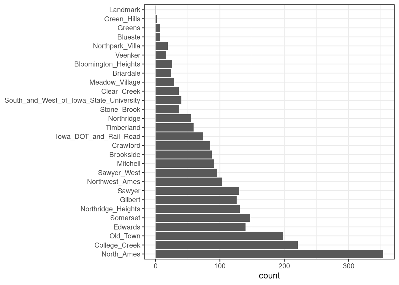
Figure 8.1: Frequencies of neighborhoods in the Ames training set
Here we see that two neighborhoods have less than five properties in the training data (Landmark and Green Hills); in this case, no houses at all in the Landmark neighborhood were included in the testing set. For some models, it may be problematic to have dummy variables with a single nonzero entry in the column. At a minimum, it is highly improbable that these features would be important to a model. If we add step_other(Neighborhood, threshold = 0.01) to our recipe, the bottom 1% of the neighborhoods will be lumped into a new level called “other.” In this training set, this will catch seven neighborhoods.
For the Ames data, we can amend the recipe to use:
simple_ames <-
  recipe(Sale_Price ~ Neighborhood + Gr_Liv_Area + Year_Built + Bldg_Type,
         data = ames_train) %>%
  step_log(Gr_Liv_Area, base = 10) %>%
  step_other(Neighborhood, threshold = 0.01) %>%
  step_dummy(all_nominal_predictors())
Many, but not all, underlying model calculations require predictor values to be encoded as numbers. Notable exceptions include tree-based models, rule-based models, and naive Bayes models.
The most common method for converting a factor predictor to a numeric format is to create dummy or indicator variables. Let’s take the predictor in the Ames data for the building type, which is a factor variable with five levels (see Table 8.1). For dummy variables, the single Bldg_Type column would be replaced with four numeric columns whose values are either zero or one. These binary variables represent specific factor level values. In R, the convention is to exclude a column for the first factor level (OneFam, in this case). The Bldg_Type column would be replaced with a column called TwoFmCon that is one when the row has that value and zero otherwise. Three other columns are similarly created:
| Raw Data | TwoFmCon | Duplex | Twnhs | TwnhsE |
|---|---|---|---|---|
| OneFam | 0 | 0 | 0 | 0 |
| TwoFmCon | 1 | 0 | 0 | 0 |
| Duplex | 0 | 1 | 0 | 0 |
| Twnhs | 0 | 0 | 1 | 0 |
| TwnhsE | 0 | 0 | 0 | 1 |
Why not all five? The most basic reason is simplicity; if you know the value for these four columns, you can determine the last value because these are mutually exclusive categories. More technically, the classical justification is that a number of models, including ordinary linear regression, have numerical issues when there are linear dependencies between columns. If all five building type indicator columns are included, they would add up to the intercept column (if there is one). This would cause an issue, or perhaps an outright error, in the underlying matrix algebra.
The full set of encodings can be used for some models. This is traditionally called the one-hot encoding and can be achieved using the one_hot argument of step_dummy().
One helpful feature of step_dummy() is that there is more control over how the resulting dummy variables are named. In base R, dummy variable names mash the variable name with the level, resulting in names like NeighborhoodVeenker. Recipes, by default, use an underscore as the separator between the name and level (e.g., Neighborhood_Veenker) and there is an option to use custom formatting for the names. The default naming convention in recipes makes it easier to capture those new columns in future steps using a selector, such as starts_with("Neighborhood_").
Traditional dummy variables require that all of the possible categories be known to create a full set of numeric features. There are other methods for doing this transformation to a numeric format. Feature hashing methods only consider the value of the category to assign it to a predefined pool of dummy variables. Effect or likelihood encodings replace the original data with a single numeric column that measures the effect of those data. Both feature hashing and effect encoding can seamlessly handle situations where a novel factor level is encountered in the data. Chapter 17 explores these and other methods for encoding categorical data, beyond straightforward dummy or indicator variables.
Different recipe steps behave differently when applied to variables in the data. For example, step_log() modifies a column in place without changing the name. Other steps, such as step_dummy(), eliminate the original data column and replace it with one or more columns with different names. The effect of a recipe step depends on the type of feature engineering transformation being done.
8.4.2 Interaction terms
Interaction effects involve two or more predictors. Such an effect occurs when one predictor has an effect on the outcome that is contingent on one or more other predictors. For example, if you were trying to predict how much traffic there will be during your commute, two potential predictors could be the specific time of day you commute and the weather. However, the relationship between the amount of traffic and bad weather is different for different times of day. In this case, you could add an interaction term between the two predictors to the model along with the original two predictors (which are called the main effects). Numerically, an interaction term between predictors is encoded as their product. Interactions are defined in terms of their effect on the outcome and can be combinations of different types of data (e.g., numeric, categorical, etc). Chapter 7 of M. Kuhn and Johnson (2020) discusses interactions and how to detect them in greater detail.
After exploring the Ames training set, we might find that the regression slopes for the gross living area differ for different building types, as shown in Figure 8.2.
ggplot(ames_train, aes(x = Gr_Liv_Area, y = 10^Sale_Price)) +
  geom_point(alpha = .2) +
  facet_wrap(~ Bldg_Type) +
  geom_smooth(method = lm, formula = y ~ x, se = FALSE, color = "lightblue") +
  scale_x_log10() +
  scale_y_log10() +
  labs(x = "Gross Living Area", y = "Sale Price (USD)")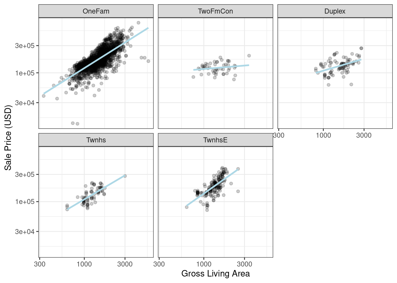
Figure 8.2: Gross living area (in log-10 units) versus sale price (also in log-10 units) for five different building types
How are interactions specified in a recipe? A base R formula would take an interaction using a :, so we would use:
Sale_Price ~ Neighborhood + log10(Gr_Liv_Area) + Bldg_Type +
  log10(Gr_Liv_Area):Bldg_Type
# or
Sale_Price ~ Neighborhood + log10(Gr_Liv_Area) * Bldg_Type
where * expands those columns to the main effects and interaction term. Again, the formula method does many things simultaneously and understands that a factor variable (such as Bldg_Type) should be expanded into dummy variables first and that the interaction should involve all of the resulting binary columns.
Recipes are more explicit and sequential, and they give you more control. With the current recipe, step_dummy() has already created dummy variables. How would we combine these for an interaction? The additional step would look like step_interact(~ interaction terms) where the terms on the right-hand side of the tilde are the interactions. These can include selectors, so it would be appropriate to use:
simple_ames <-
  recipe(Sale_Price ~ Neighborhood + Gr_Liv_Area + Year_Built + Bldg_Type,
         data = ames_train) %>%
  step_log(Gr_Liv_Area, base = 10) %>%
  step_other(Neighborhood, threshold = 0.01) %>%
  step_dummy(all_nominal_predictors()) %>%
  # Gr_Liv_Area is on the log scale from a previous step
  step_interact( ~ Gr_Liv_Area:starts_with("Bldg_Type_") )
Additional interactions can be specified in this formula by separating them by +. Also note that the recipe will only use interactions between different variables; if the formula uses var_1:var_1, this term will be ignored.
Suppose that, in a recipe, we had not yet made dummy variables for building types. It would be inappropriate to include a factor column in this step, such as:
step_interact( ~ Gr_Liv_Area:Bldg_Type )This is telling the underlying (base R) code used by step_interact() to make dummy variables and then form the interactions. In fact, if this occurs, a warning states that this might generate unexpected results.
This behavior gives you more control, but it is different from R’s standard model formula.
As with naming dummy variables, recipes provides more coherent names for interaction terms. In this case, the interaction is named Gr_Liv_Area_x_Bldg_Type_Duplex instead of Gr_Liv_Area:Bldg_TypeDuplex (which is not a valid column name for a data frame).
Remember that order matters. The gross living area is log transformed prior to the interaction term. Subsequent interactions with this variable will also use the log scale.
8.4.3 Spline functions
When a predictor has a nonlinear relationship with the outcome, some types of predictive models can adaptively approximate this relationship during training. However, simpler is usually better and it is not uncommon to try to use a simple model, such as a linear fit, and add in specific nonlinear features for predictors that may need them, such as longitude and latitude for the Ames housing data. One common method for doing this is to use spline functions to represent the data. Splines replace the existing numeric predictor with a set of columns that allow a model to emulate a flexible, nonlinear relationship. As more spline terms are added to the data, the capacity to nonlinearly represent the relationship increases. Unfortunately, it may also increase the likelihood of picking up on data trends that occur by chance (i.e., overfitting).
If you have ever used geom_smooth() within a ggplot, you have probably used a spline representation of the data. For example, each panel in Figure 8.3 uses a different number of smooth splines for the latitude predictor:
library(patchwork)
library(splines)

plot_smoother <- function(deg_free) {
  ggplot(ames_train, aes(x = Latitude, y = 10^Sale_Price)) +
    geom_point(alpha = .2) +
    scale_y_log10() +
    geom_smooth(
      method = lm,
      formula = y ~ ns(x, df = deg_free),
      color = "lightblue",
      se = FALSE
    ) +
    labs(title = paste(deg_free, "Spline Terms"),
         y = "Sale Price (USD)")
}

( plot_smoother(2) + plot_smoother(5) ) / ( plot_smoother(20) + plot_smoother(100) )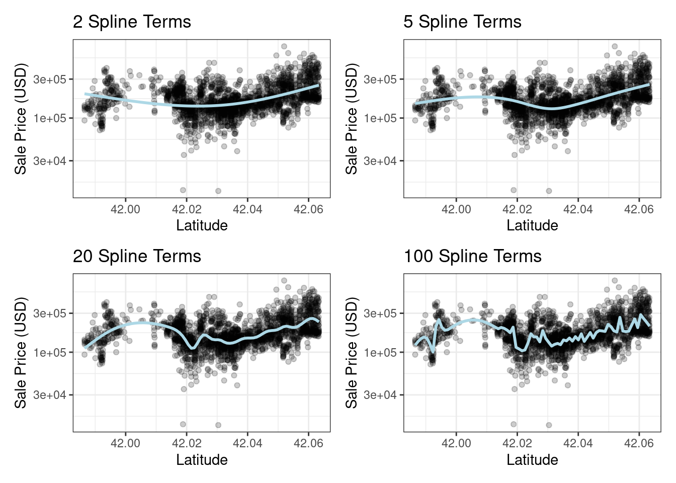
Figure 8.3: Sale price versus latitude, with trend lines using natural splines with different degrees of freedom
The ns() function in the splines package generates feature columns using functions called natural splines.
Some panels in Figure 8.3 clearly fit poorly; two terms underfit the data while 100 terms overfit. The panels with five and twenty terms seem like reasonably smooth fits that catch the main patterns of the data. This indicates that the proper amount of “nonlinear-ness” matters. The number of spline terms could then be considered a tuning parameter for this model. These types of parameters are explored in Chapter 12.
In recipes, multiple steps can create these types of terms. To add a natural spline representation for this predictor:
recipe(Sale_Price ~ Neighborhood + Gr_Liv_Area + Year_Built + Bldg_Type + Latitude,
         data = ames_train) %>%
  step_log(Gr_Liv_Area, base = 10) %>%
  step_other(Neighborhood, threshold = 0.01) %>%
  step_dummy(all_nominal_predictors()) %>%
  step_interact( ~ Gr_Liv_Area:starts_with("Bldg_Type_") ) %>%
  step_ns(Latitude, deg_free = 20)
The user would need to determine if both neighborhood and latitude should be in the model since they both represent the same underlying data in different ways.
8.4.4 Feature extraction
Another common method for representing multiple features at once is called feature extraction. Most of these techniques create new features from the predictors that capture the information in the broader set as a whole. For example, principal component analysis (PCA) tries to extract as much of the original information in the predictor set as possible using a smaller number of features. PCA is a linear extraction method, meaning that each new feature is a linear combination of the original predictors. One nice aspect of PCA is that each of the new features, called the principal components or PCA scores, are uncorrelated with one another. Because of this, PCA can be very effective at reducing the correlation between predictors. Note that PCA is only aware of the predictors; the new PCA features might not be associated with the outcome.
In the Ames data, several predictors measure size of the property, such as the total basement size (Total_Bsmt_SF), size of the first floor (First_Flr_SF), the gross living area (Gr_Liv_Area), and so on. PCA might be an option to represent these potentially redundant variables as a smaller feature set. Apart from the gross living area, these predictors have the suffix SF in their names (for square feet) so a recipe step for PCA might look like:
  # Use a regular expression to capture house size predictors:
  step_pca(matches("(SF$)|(Gr_Liv)"))
Note that all of these columns are measured in square feet. PCA assumes that all of the predictors are on the same scale. That’s true in this case, but often this step can be preceded by step_normalize(), which will center and scale each column.
There are existing recipe steps for other extraction methods, such as: independent component analysis (ICA), non-negative matrix factorization (NNMF), multidimensional scaling (MDS), uniform manifold approximation and projection (UMAP), and others.
8.4.5 Row sampling steps
Recipe steps can affect the rows of a data set as well. For example, subsampling techniques for class imbalances change the class proportions in the data being given to the model; these techniques often don’t improve overall performance but can generate better behaved distributions of the predicted class probabilities. These are approaches to try when subsampling your data with class imbalance:
Downsampling the data keeps the minority class and takes a random sample of the majority class so that class frequencies are balanced.
Upsampling replicates samples from the minority class to balance the classes. Some techniques do this by synthesizing new samples that resemble the minority class data while other methods simply add the same minority samples repeatedly.
Hybrid methods do a combination of both.
The themis package has recipe steps that can be used to address class imbalance via subsampling. For simple downsampling, we would use:
step_downsample(outcome_column_name)Only the training set should be affected by these techniques. The test set or other holdout samples should be left as-is when processed using the recipe. For this reason, all of the subsampling steps default the skip argument to have a value of TRUE (Section 8.5).
Other step functions are row-based as well: step_filter(), step_sample(), step_slice(), and step_arrange(). In almost all uses of these steps, the skip argument should be set to TRUE.
8.4.6 General transformations
Mirroring the original dplyr operation, step_mutate() can be used to conduct a variety of basic operations to the data. It is best used for straightforward transformations like computing a ratio of two variables, such as Bedroom_AbvGr / Full_Bath, the ratio of bedrooms to bathrooms for the Ames housing data.
When using this flexible step, use extra care to avoid data leakage in your preprocessing. Consider, for example, the transformation x = w > mean(w). When applied to new data or testing data, this transformation would use the mean of w from the new data, not the mean of w from the training data.
8.4.7 Natural language processing
Recipes can also handle data that are not in the traditional structure where the columns are features. For example, the textrecipes package can apply natural language processing methods to the data. The input column is typically a string of text, and different steps can be used to tokenize the data (e.g., split the text into separate words), filter out tokens, and create new features appropriate for modeling.
8.5 Skipping Steps for New Data
The sale price data are already log-transformed in the ames data frame. Why not use:
step_log(Sale_Price, base = 10)This will cause a failure when the recipe is applied to new properties with an unknown sale price. Since price is what we are trying to predict, there probably won’t be a column in the data for this variable. In fact, to avoid information leakage, many tidymodels packages isolate the data being used when making any predictions. This means that the training set and any outcome columns are not available for use at prediction time.
For simple transformations of the outcome column(s), we strongly suggest that those operations be conducted outside of the recipe.
However, there are other circumstances where this is not an adequate solution. For example, in classification models where there is a severe class imbalance, it is common to conduct subsampling of the data that are given to the modeling function. For example, suppose that there were two classes and a 10% event rate. A simple, albeit controversial, approach would be to downsample the data so that the model is provided with all of the events and a random 10% of the nonevent samples.
The problem is that the same subsampling process should not be applied to the data being predicted. As a result, when using a recipe, we need a mechanism to ensure that some operations are applied only to the data that are given to the model. Each step function has an option called skip that, when set to TRUE, will be ignored by the predict() function. In this way, you can isolate the steps that affect the modeling data without causing errors when applied to new samples. However, all steps are applied when using fit().
At the time of this writing, the step functions in the recipes and themis packages that are only applied to the training data are: step_adasyn(), step_bsmote(), step_downsample(), step_filter(), step_naomit(), step_nearmiss(), step_rose(), step_sample(), step_slice(), step_smote(), step_smotenc(), step_tomek(), and step_upsample().
8.6 Tidy a recipe()
In Section 3.3, we introduced the tidy() verb for statistical objects. There is also a tidy() method for recipes, as well as individual recipe steps. Before proceeding, let’s create an extended recipe for the Ames data using some of the new steps we’ve discussed in this chapter:
ames_rec <-
  recipe(Sale_Price ~ Neighborhood + Gr_Liv_Area + Year_Built + Bldg_Type +
           Latitude + Longitude, data = ames_train) %>%
  step_log(Gr_Liv_Area, base = 10) %>%
  step_other(Neighborhood, threshold = 0.01) %>%
  step_dummy(all_nominal_predictors()) %>%
  step_interact( ~ Gr_Liv_Area:starts_with("Bldg_Type_") ) %>%
  step_ns(Latitude, Longitude, deg_free = 20)
The tidy() method, when called with the recipe object, gives a summary of the recipe steps:
tidy(ames_rec)
#> # A tibble: 5 × 6
#>   number operation type     trained skip  id
#>    <int> <chr>     <chr>    <lgl>   <lgl> <chr>
#> 1      1 step      log      FALSE   FALSE log_66JTU
#> 2      2 step      other    FALSE   FALSE other_ePfcw
#> 3      3 step      dummy    FALSE   FALSE dummy_Z18Cl
#> 4      4 step      interact FALSE   FALSE interact_JLU36
#> 5      5 step      ns       FALSE   FALSE ns_rvsqQ
This result can be helpful for identifying individual steps, perhaps to then be able to execute the tidy() method on one specific step.
We can specify the id argument in any step function call; otherwise it is generated using a random suffix. Setting this value can be helpful if the same type of step is added to the recipe more than once. Let’s specify the id ahead of time for step_other(), since we’ll want to tidy() it:
ames_rec <-
  recipe(Sale_Price ~ Neighborhood + Gr_Liv_Area + Year_Built + Bldg_Type +
           Latitude + Longitude, data = ames_train) %>%
  step_log(Gr_Liv_Area, base = 10) %>%
  step_other(Neighborhood, threshold = 0.01, id = "my_id") %>%
  step_dummy(all_nominal_predictors()) %>%
  step_interact( ~ Gr_Liv_Area:starts_with("Bldg_Type_") ) %>%
  step_ns(Latitude, Longitude, deg_free = 20)
We’ll refit the workflow with this new recipe:
lm_wflow <-
  workflow() %>%
  add_model(lm_model) %>%
  add_recipe(ames_rec)

lm_fit <- fit(lm_wflow, ames_train)
The tidy() method can be called again along with the id identifier we specified to get our results for applying step_other():
estimated_recipe <-
  lm_fit %>%
  extract_recipe(estimated = TRUE)

tidy(estimated_recipe, id = "my_id")
#> # A tibble: 22 × 3
#>   terms        retained           id
#>   <chr>        <chr>              <chr>
#> 1 Neighborhood North_Ames         my_id
#> 2 Neighborhood College_Creek      my_id
#> 3 Neighborhood Old_Town           my_id
#> 4 Neighborhood Edwards            my_id
#> 5 Neighborhood Somerset           my_id
#> 6 Neighborhood Northridge_Heights my_id
#> # ℹ 16 more rows
The tidy() results we see here for using step_other() show which factor levels were retained, i.e., not added to the new “other” category.
The tidy() method can be called with the number identifier as well, if we know which step in the recipe we need:
tidy(estimated_recipe, number = 2)
#> # A tibble: 22 × 3
#>   terms        retained           id
#>   <chr>        <chr>              <chr>
#> 1 Neighborhood North_Ames         my_id
#> 2 Neighborhood College_Creek      my_id
#> 3 Neighborhood Old_Town           my_id
#> 4 Neighborhood Edwards            my_id
#> 5 Neighborhood Somerset           my_id
#> 6 Neighborhood Northridge_Heights my_id
#> # ℹ 16 more rows
Each tidy() method returns the relevant information about that step. For example, the tidy() method for step_dummy() returns a column with the variables that were converted to dummy variables and another column with all of the known levels for each column.
8.7 Column Roles
When a formula is used with the initial call to recipe() it assigns roles to each of the columns, depending on which side of the tilde they are on. Those roles are either "predictor" or "outcome". However, other roles can be assigned as needed.
For example, in our Ames data set, the original raw data contained a column for address.17 It may be useful to keep that column in the data so that, after predictions are made, problematic results can be investigated in detail. In other words, the column could be important even when it isn’t a predictor or outcome.
To solve this, the add_role(), remove_role(), and update_role() functions can be helpful. For example, for the house price data, the role of the street address column could be modified using:
ames_rec %>% update_role(address, new_role = "street address")After this change, the address column in the dataframe will no longer be a predictor but instead will be a "street address" according to the recipe. Any character string can be used as a role. Also, columns can have multiple roles (additional roles are added via add_role()) so that they can be selected under more than one context.
This can be helpful when the data are resampled. It helps to keep the columns that are not involved with the model fit in the same data frame (rather than in an external vector). Resampling, described in Chapter 10, creates alternate versions of the data mostly by row subsampling. If the street address were in another column, additional subsampling would be required and might lead to more complex code and a higher likelihood of errors.
Finally, all step functions have a role field that can assign roles to the results of the step. In many cases, columns affected by a step retain their existing role. For example, the step_log() calls to our ames_rec object affected the Gr_Liv_Area column. For that step, the default behavior is to keep the existing role for this column since no new column is created. As a counter-example, the step to produce splines defaults new columns to have a role of "predictor" since that is usually how spline columns are used in a model. Most steps have sensible defaults but, since the defaults can be different, be sure to check the documentation page to understand which role(s) will be assigned.
8.8 Chapter Summary
In this chapter, you learned about using recipes for flexible feature engineering and data preprocessing, from creating dummy variables to handling class imbalance and more. Feature engineering is an important part of the modeling process where information leakage can easily occur and good practices must be adopted. Between the recipes package and other packages that extend recipes, there are over 100 available steps. All possible recipe steps are enumerated at tidymodels.org/find. The recipes framework provides a rich data manipulation environment for preprocessing and transforming data prior to modeling.
Additionally, tidymodels.org/learn/develop/recipes/ shows how custom steps can be created.
Our work here has used recipes solely inside of a workflow object. For modeling, that is the recommended use because feature engineering should be estimated together with a model. However, for visualization and other activities, a workflow may not be appropriate; more recipe-specific functions may be required. Chapter 16 discusses lower-level APIs for fitting, using, and troubleshooting recipes.
The code that we will use in later chapters is:
library(tidymodels)
data(ames)
ames <- mutate(ames, Sale_Price = log10(Sale_Price))

set.seed(502)
ames_split <- initial_split(ames, prop = 0.80, strata = Sale_Price)
ames_train <- training(ames_split)
ames_test  <-  testing(ames_split)

ames_rec <-
  recipe(Sale_Price ~ Neighborhood + Gr_Liv_Area + Year_Built + Bldg_Type +
           Latitude + Longitude, data = ames_train) %>%
  step_log(Gr_Liv_Area, base = 10) %>%
  step_other(Neighborhood, threshold = 0.01) %>%
  step_dummy(all_nominal_predictors()) %>%
  step_interact( ~ Gr_Liv_Area:starts_with("Bldg_Type_") ) %>%
  step_ns(Latitude, Longitude, deg_free = 20)

lm_model <- linear_reg() %>% set_engine("lm")

lm_wflow <-
  workflow() %>%
  add_model(lm_model) %>%
  add_recipe(ames_rec)

lm_fit <- fit(lm_wflow, ames_train)
REFERENCES
Our version of these data does not contain that column.↩︎