15 Screening Many Models
We introduced workflow sets in Chapter 7 and demonstrated how to use them with resampled data sets in Chapter 11. In this chapter, we discuss these sets of multiple modeling workflows in more detail and describe a use case where they can be helpful.
For projects with new data sets that have not yet been well understood, a data practitioner may need to screen many combinations of models and preprocessors. It is common to have little or no a priori knowledge about which method will work best with a novel data set.
A good strategy is to spend some initial effort trying a variety of modeling approaches, determine what works best, then invest additional time tweaking/optimizing a small set of models.
Workflow sets provide a user interface to create and manage this process. We’ll also demonstrate how to evaluate these models efficiently using the racing methods discussed in Section 15.4.
15.1 Modeling Concrete Mixture Strength
To demonstrate how to screen multiple model workflows, we will use the concrete mixture data from Applied Predictive Modeling (M. Kuhn and Johnson 2013) as an example. Chapter 10 of that book demonstrated models to predict the compressive strength of concrete mixtures using the ingredients as predictors. A wide variety of models were evaluated with different predictor sets and preprocessing needs. How can workflow sets make such a process of large scale testing for models easier?
First, let’s define the data splitting and resampling schemes.
library(tidymodels)
tidymodels_prefer()
data(concrete, package = "modeldata")
glimpse(concrete)
#> Rows: 1,030
#> Columns: 9
#> $ cement               <dbl> 540.0, 540.0, 332.5, 332.5, 198.6, 266.0, 380.0, 380.…
#> $ blast_furnace_slag   <dbl> 0.0, 0.0, 142.5, 142.5, 132.4, 114.0, 95.0, 95.0, 114…
#> $ fly_ash              <dbl> 0, 0, 0, 0, 0, 0, 0, 0, 0, 0, 0, 0, 0, 0, 0, 0, 0, 0,…
#> $ water                <dbl> 162, 162, 228, 228, 192, 228, 228, 228, 228, 228, 192…
#> $ superplasticizer     <dbl> 2.5, 2.5, 0.0, 0.0, 0.0, 0.0, 0.0, 0.0, 0.0, 0.0, 0.0…
#> $ coarse_aggregate     <dbl> 1040.0, 1055.0, 932.0, 932.0, 978.4, 932.0, 932.0, 93…
#> $ fine_aggregate       <dbl> 676.0, 676.0, 594.0, 594.0, 825.5, 670.0, 594.0, 594.…
#> $ age                  <int> 28, 28, 270, 365, 360, 90, 365, 28, 28, 28, 90, 28, 2…
#> $ compressive_strength <dbl> 79.99, 61.89, 40.27, 41.05, 44.30, 47.03, 43.70, 36.4…
The compressive_strength column is the outcome. The age predictor tells us the age of the concrete sample at testing in days (concrete strengthens over time) and the rest of the predictors like cement and water are concrete components in units of kilograms per cubic meter.
For some cases in this data set, the same concrete formula was tested multiple times. We’d rather not include these replicate mixtures as individual data points since they might be distributed across both the training and test set. Doing so might artificially inflate our performance estimates.
To address this, we will use the mean compressive strength per concrete mixture for modeling:
concrete <-
   concrete %>%
   group_by(across(-compressive_strength)) %>%
   summarize(compressive_strength = mean(compressive_strength),
             .groups = "drop")
nrow(concrete)
#> [1] 992
Let’s split the data using the default 3:1 ratio of training-to-test and resample the training set using five repeats of 10-fold cross-validation:
set.seed(1501)
concrete_split <- initial_split(concrete, strata = compressive_strength)
concrete_train <- training(concrete_split)
concrete_test  <- testing(concrete_split)

set.seed(1502)
concrete_folds <-
   vfold_cv(concrete_train, strata = compressive_strength, repeats = 5)
Some models (notably neural networks, KNN, and support vector machines) require predictors that have been centered and scaled, so some model workflows will require recipes with these preprocessing steps. For other models, a traditional response surface design model expansion (i.e., quadratic and two-way interactions) is a good idea. For these purposes, we create two recipes:
normalized_rec <-
   recipe(compressive_strength ~ ., data = concrete_train) %>%
   step_normalize(all_predictors())

poly_recipe <-
   normalized_rec %>%
   step_poly(all_predictors()) %>%
   step_interact(~ all_predictors():all_predictors())
For the models, we use the the parsnip addin to create a set of model specifications:
library(rules)
library(baguette)

linear_reg_spec <-
   linear_reg(penalty = tune(), mixture = tune()) %>%
   set_engine("glmnet")

nnet_spec <-
   mlp(hidden_units = tune(), penalty = tune(), epochs = tune()) %>%
   set_engine("nnet", MaxNWts = 2600) %>%
   set_mode("regression")

mars_spec <-
   mars(prod_degree = tune()) %>%  #<- use GCV to choose terms
   set_engine("earth") %>%
   set_mode("regression")

svm_r_spec <-
   svm_rbf(cost = tune(), rbf_sigma = tune()) %>%
   set_engine("kernlab") %>%
   set_mode("regression")

svm_p_spec <-
   svm_poly(cost = tune(), degree = tune()) %>%
   set_engine("kernlab") %>%
   set_mode("regression")

knn_spec <-
   nearest_neighbor(neighbors = tune(), dist_power = tune(), weight_func = tune()) %>%
   set_engine("kknn") %>%
   set_mode("regression")

cart_spec <-
   decision_tree(cost_complexity = tune(), min_n = tune()) %>%
   set_engine("rpart") %>%
   set_mode("regression")

bag_cart_spec <-
   bag_tree() %>%
   set_engine("rpart", times = 50L) %>%
   set_mode("regression")

rf_spec <-
   rand_forest(mtry = tune(), min_n = tune(), trees = 1000) %>%
   set_engine("ranger") %>%
   set_mode("regression")

xgb_spec <-
   boost_tree(tree_depth = tune(), learn_rate = tune(), loss_reduction = tune(),
              min_n = tune(), sample_size = tune(), trees = tune()) %>%
   set_engine("xgboost") %>%
   set_mode("regression")

cubist_spec <-
   cubist_rules(committees = tune(), neighbors = tune()) %>%
   set_engine("Cubist")
The analysis in M. Kuhn and Johnson (2013) specifies that the neural network should have up to 27 hidden units in the layer. The extract_parameter_set_dials() function extracts the parameter set, which we modify to have the correct parameter range:
nnet_param <-
   nnet_spec %>%
   extract_parameter_set_dials() %>%
   update(hidden_units = hidden_units(c(1, 27)))
How can we match these models to their recipes, tune them, then evaluate their performance efficiently? A workflow set offers a solution.
15.2 Creating the Workflow Set
Workflow sets take named lists of preprocessors and model specifications and combine them into an object containing multiple workflows. There are three possible kinds of preprocessors:
- A standard R formula
- A recipe object (prior to estimation/prepping)
- A dplyr-style selector to choose the outcome and predictors
As a first workflow set example, let’s combine the recipe that only standardizes the predictors to the nonlinear models that require the predictors to be in the same units:
normalized <-
   workflow_set(
      preproc = list(normalized = normalized_rec),
      models = list(SVM_radial = svm_r_spec, SVM_poly = svm_p_spec,
                    KNN = knn_spec, neural_network = nnet_spec)
   )
normalized
#> # A workflow set/tibble: 4 × 4
#>   wflow_id                  info             option    result
#>   <chr>                     <list>           <list>    <list>
#> 1 normalized_SVM_radial     <tibble [1 × 4]> <opts[0]> <list [0]>
#> 2 normalized_SVM_poly       <tibble [1 × 4]> <opts[0]> <list [0]>
#> 3 normalized_KNN            <tibble [1 × 4]> <opts[0]> <list [0]>
#> 4 normalized_neural_network <tibble [1 × 4]> <opts[0]> <list [0]>
Since there is only a single preprocessor, this function creates a set of workflows with this value. If the preprocessor contained more than one entry, the function would create all combinations of preprocessors and models.
The wflow_id column is automatically created but can be modified using a call to mutate(). The info column contains a tibble with some identifiers and the workflow object. The workflow can be extracted:
normalized %>% extract_workflow(id = "normalized_KNN")
#> ══ Workflow ═════════════════════════════════════════════════════════════════════════
#> Preprocessor: Recipe
#> Model: nearest_neighbor()
#>
#> ── Preprocessor ─────────────────────────────────────────────────────────────────────
#> 1 Recipe Step
#>
#> • step_normalize()
#>
#> ── Model ────────────────────────────────────────────────────────────────────────────
#> K-Nearest Neighbor Model Specification (regression)
#>
#> Main Arguments:
#>   neighbors = tune()
#>   weight_func = tune()
#>   dist_power = tune()
#>
#> Computational engine: kknn
The option column is a placeholder for any arguments to use when we evaluate the workflow. For example, to add the neural network parameter object:
normalized <-
   normalized %>%
   option_add(param_info = nnet_param, id = "normalized_neural_network")
normalized
#> # A workflow set/tibble: 4 × 4
#>   wflow_id                  info             option    result
#>   <chr>                     <list>           <list>    <list>
#> 1 normalized_SVM_radial     <tibble [1 × 4]> <opts[0]> <list [0]>
#> 2 normalized_SVM_poly       <tibble [1 × 4]> <opts[0]> <list [0]>
#> 3 normalized_KNN            <tibble [1 × 4]> <opts[0]> <list [0]>
#> 4 normalized_neural_network <tibble [1 × 4]> <opts[1]> <list [0]>
When a function from the tune or finetune package is used to tune (or resample) the workflow, this argument will be used.
The result column is a placeholder for the output of the tuning or resampling functions.
For the other nonlinear models, let’s create another workflow set that uses dplyr selectors for the outcome and predictors:
model_vars <-
   workflow_variables(outcomes = compressive_strength,
                      predictors = everything())

no_pre_proc <-
   workflow_set(
      preproc = list(simple = model_vars),
      models = list(MARS = mars_spec, CART = cart_spec, CART_bagged = bag_cart_spec,
                    RF = rf_spec, boosting = xgb_spec, Cubist = cubist_spec)
   )
no_pre_proc
#> # A workflow set/tibble: 6 × 4
#>   wflow_id           info             option    result
#>   <chr>              <list>           <list>    <list>
#> 1 simple_MARS        <tibble [1 × 4]> <opts[0]> <list [0]>
#> 2 simple_CART        <tibble [1 × 4]> <opts[0]> <list [0]>
#> 3 simple_CART_bagged <tibble [1 × 4]> <opts[0]> <list [0]>
#> 4 simple_RF          <tibble [1 × 4]> <opts[0]> <list [0]>
#> 5 simple_boosting    <tibble [1 × 4]> <opts[0]> <list [0]>
#> 6 simple_Cubist      <tibble [1 × 4]> <opts[0]> <list [0]>
Finally, we assemble the set that uses nonlinear terms and interactions with the appropriate models:
with_features <-
   workflow_set(
      preproc = list(full_quad = poly_recipe),
      models = list(linear_reg = linear_reg_spec, KNN = knn_spec)
   )
These objects are tibbles with the extra class of workflow_set. Row binding does not affect the state of the sets and the result is itself a workflow set:
all_workflows <-
   bind_rows(no_pre_proc, normalized, with_features) %>%
   # Make the workflow ID's a little more simple:
   mutate(wflow_id = gsub("(simple_)|(normalized_)", "", wflow_id))
all_workflows
#> # A workflow set/tibble: 12 × 4
#>   wflow_id    info             option    result
#>   <chr>       <list>           <list>    <list>
#> 1 MARS        <tibble [1 × 4]> <opts[0]> <list [0]>
#> 2 CART        <tibble [1 × 4]> <opts[0]> <list [0]>
#> 3 CART_bagged <tibble [1 × 4]> <opts[0]> <list [0]>
#> 4 RF          <tibble [1 × 4]> <opts[0]> <list [0]>
#> 5 boosting    <tibble [1 × 4]> <opts[0]> <list [0]>
#> 6 Cubist      <tibble [1 × 4]> <opts[0]> <list [0]>
#> # ℹ 6 more rows
15.3 Tuning and Evaluating the Models
Almost all of the members of all_workflows contain tuning parameters. To evaluate their performance, we can use the standard tuning or resampling functions (e.g., tune_grid() and so on). The workflow_map() function will apply the same function to all of the workflows in the set; the default is tune_grid().
For this example, grid search is applied to each workflow using up to 25 different parameter candidates. There are a set of common options to use with each execution of tune_grid(). For example, in the following code we will use the same resampling and control objects for each workflow, along with a grid size of 25. The workflow_map() function has an additional argument called seed, which is used to ensure that each execution of tune_grid() consumes the same random numbers.
grid_ctrl <-
   control_grid(
      save_pred = TRUE,
      parallel_over = "everything",
      save_workflow = TRUE
   )

grid_results <-
   all_workflows %>%
   workflow_map(
      seed = 1503,
      resamples = concrete_folds,
      grid = 25,
      control = grid_ctrl
   )
The results show that the option and result columns have been updated:
grid_results
#> # A workflow set/tibble: 12 × 4
#>   wflow_id    info             option    result
#>   <chr>       <list>           <list>    <list>
#> 1 MARS        <tibble [1 × 4]> <opts[3]> <tune[+]>
#> 2 CART        <tibble [1 × 4]> <opts[3]> <tune[+]>
#> 3 CART_bagged <tibble [1 × 4]> <opts[3]> <rsmp[+]>
#> 4 RF          <tibble [1 × 4]> <opts[3]> <tune[+]>
#> 5 boosting    <tibble [1 × 4]> <opts[3]> <tune[+]>
#> 6 Cubist      <tibble [1 × 4]> <opts[3]> <tune[+]>
#> # ℹ 6 more rows
The option column now contains all of the options that we used in the workflow_map() call. This makes our results reproducible. In the result columns, the “tune[+]” and “rsmp[+]” notations mean that the object had no issues. A value such as “tune[x]” occurs if all of the models failed for some reason.
There are a few convenience functions for examining results such as grid_results. The rank_results() function will order the models by some performance metric. By default, it uses the first metric in the metric set (RMSE in this instance). Let’s filter() to look only at RMSE:
grid_results %>%
   rank_results() %>%
   filter(.metric == "rmse") %>%
   select(model, .config, rmse = mean, rank)
#> # A tibble: 252 × 4
#>   model      .config                rmse  rank
#>   <chr>      <chr>                 <dbl> <int>
#> 1 boost_tree Preprocessor1_Model04  4.25     1
#> 2 boost_tree Preprocessor1_Model06  4.29     2
#> 3 boost_tree Preprocessor1_Model13  4.31     3
#> 4 boost_tree Preprocessor1_Model14  4.39     4
#> 5 boost_tree Preprocessor1_Model16  4.46     5
#> 6 boost_tree Preprocessor1_Model03  4.47     6
#> # ℹ 246 more rows
Also by default, the function ranks all of the candidate sets; that’s why the same model can show up multiple times in the output. An option, called select_best, can be used to rank the models using their best tuning parameter combination.
The autoplot() method plots the rankings; it also has a select_best argument. The plot in Figure 15.1 visualizes the best results for each model and is generated with:
autoplot(
   grid_results,
   rank_metric = "rmse",  # <- how to order models
   metric = "rmse",       # <- which metric to visualize
   select_best = TRUE     # <- one point per workflow
) +
   geom_text(aes(y = mean - 1/2, label = wflow_id), angle = 90, hjust = 1) +
   lims(y = c(3.5, 9.5)) +
   theme(legend.position = "none")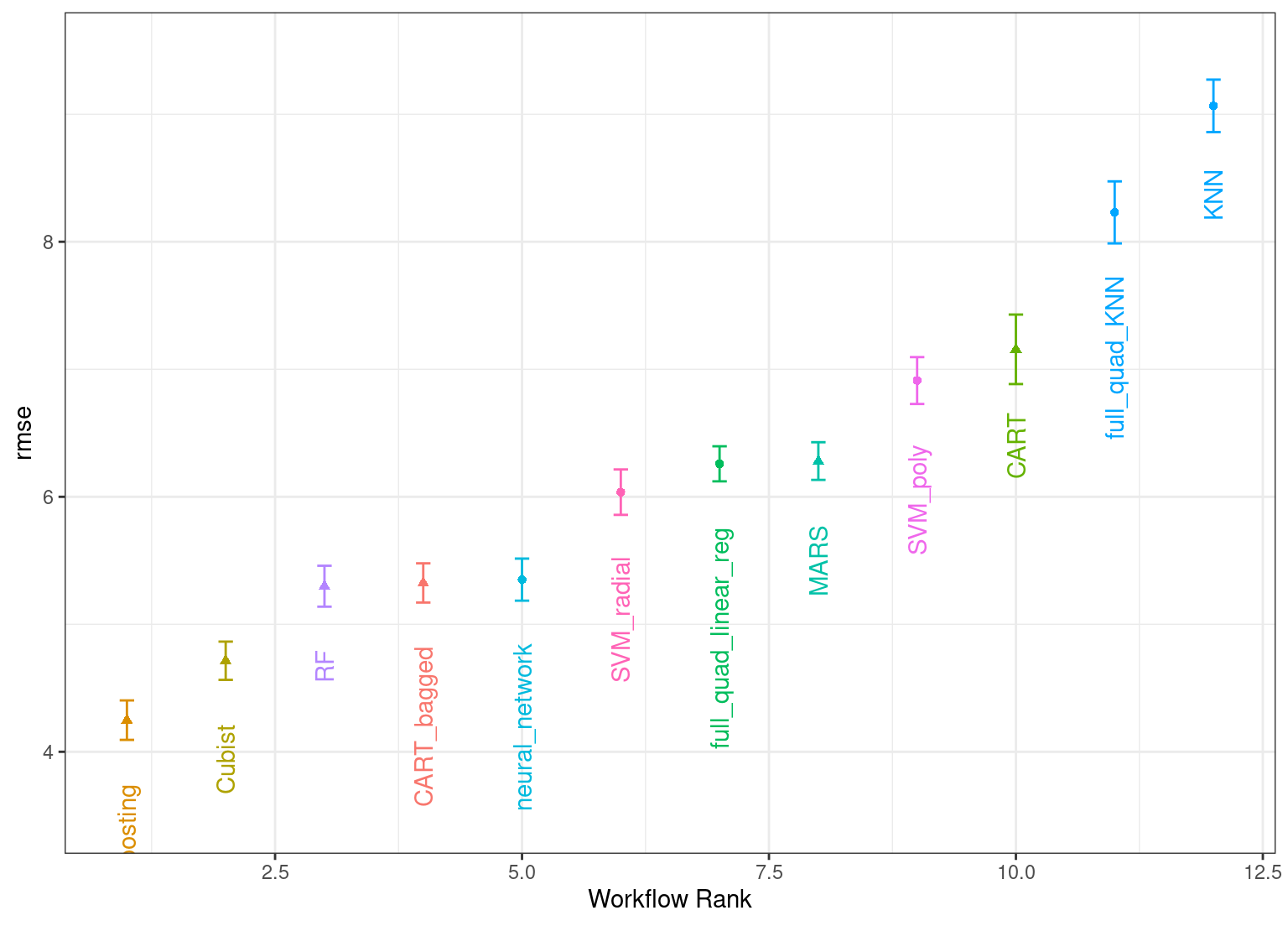
Figure 15.1: Estimated RMSE (and approximate confidence intervals) for the best model configuration in each workflow.
In case you want to see the tuning parameter results for a specific model, like Figure 15.2, the id argument can take a single value from the wflow_id column for which model to plot:
autoplot(grid_results, id = "Cubist", metric = "rmse")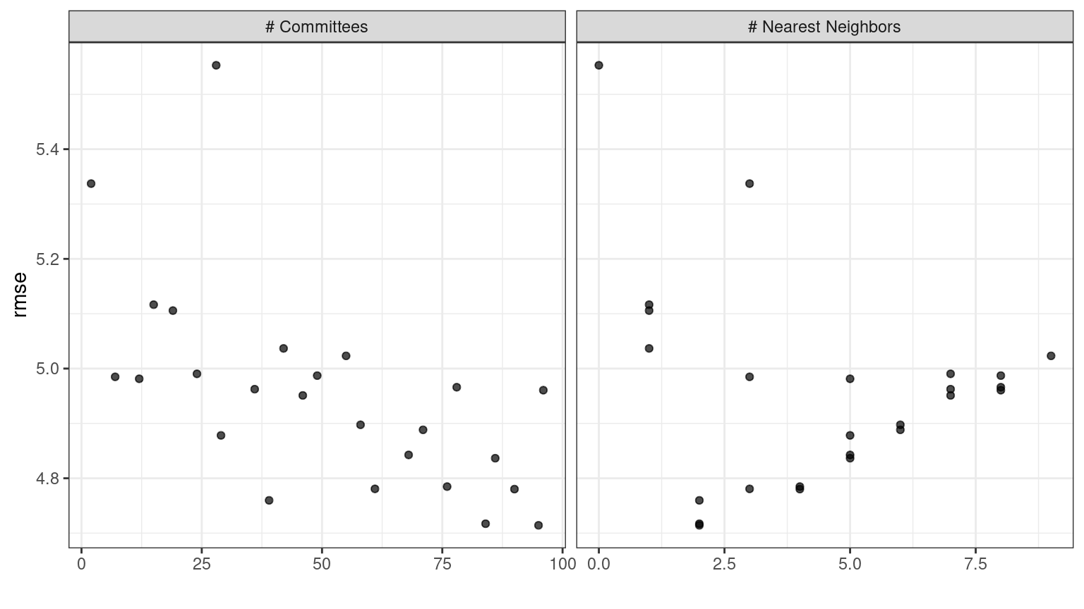
Figure 15.2: The autoplot() results for the Cubist model contained in the workflow set.
There are also methods for collect_predictions() and collect_metrics().
The example model screening with our concrete mixture data fits a total of 12,600 models. Using 2 workers in parallel, the estimation process took 1.9 hours to complete.
15.4 Efficiently Screening Models
One effective method for screening a large set of models efficiently is to use the racing approach described in Section 13.5.5. With a workflow set, we can use the workflow_map() function for this racing approach. Recall that after we pipe in our workflow set, the argument we use is the function to apply to the workflows; in this case, we can use a value of "tune_race_anova". We also pass an appropriate control object; otherwise the options would be the same as the code in the previous section.
library(finetune)

race_ctrl <-
   control_race(
      save_pred = TRUE,
      parallel_over = "everything",
      save_workflow = TRUE
   )

race_results <-
   all_workflows %>%
   workflow_map(
      "tune_race_anova",
      seed = 1503,
      resamples = concrete_folds,
      grid = 25,
      control = race_ctrl
   )
The new object looks very similar, although the elements of the result column show a value of "race[+]", indicating a different type of object:
race_results
#> # A workflow set/tibble: 12 × 4
#>   wflow_id    info             option    result
#>   <chr>       <list>           <list>    <list>
#> 1 MARS        <tibble [1 × 4]> <opts[3]> <race[+]>
#> 2 CART        <tibble [1 × 4]> <opts[3]> <race[+]>
#> 3 CART_bagged <tibble [1 × 4]> <opts[3]> <rsmp[+]>
#> 4 RF          <tibble [1 × 4]> <opts[3]> <race[+]>
#> 5 boosting    <tibble [1 × 4]> <opts[3]> <race[+]>
#> 6 Cubist      <tibble [1 × 4]> <opts[3]> <race[+]>
#> # ℹ 6 more rows
The same helpful functions are available for this object to interrogate the results and, in fact, the basic autoplot() method shown in Figure 15.331 produces trends similar to Figure 15.1. This is produced by:
autoplot(
   race_results,
   rank_metric = "rmse",
   metric = "rmse",
   select_best = TRUE
) +
   geom_text(aes(y = mean - 1/2, label = wflow_id), angle = 90, hjust = 1) +
   lims(y = c(3.0, 9.5)) +
   theme(legend.position = "none")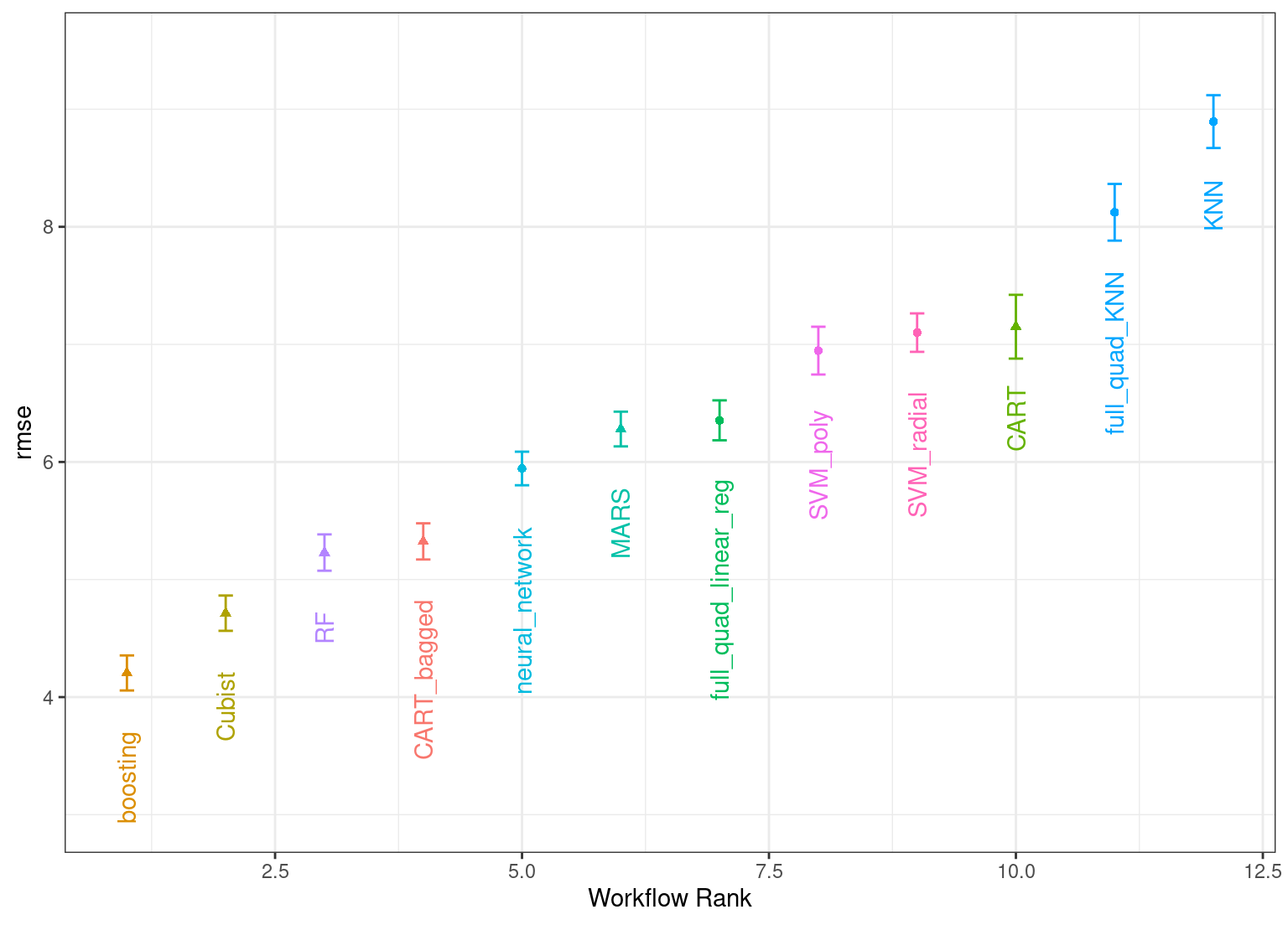
Figure 15.3: Estimated RMSE (and approximate confidence intervals) for the best model configuration in each workflow in the racing results.
Overall, the racing approach estimated a total of 1,050 models, 8.33% of the full set of 12,600 models in the full grid. As a result, the racing approach was 4.8-fold faster.
Did we get similar results? For both objects, we rank the results, merge them, and plot them against one another in Figure 15.4.
matched_results <-
   rank_results(race_results, select_best = TRUE) %>%
   select(wflow_id, .metric, race = mean, config_race = .config) %>%
   inner_join(
      rank_results(grid_results, select_best = TRUE) %>%
         select(wflow_id, .metric, complete = mean,
                config_complete = .config, model),
      by = c("wflow_id", ".metric"),
   ) %>%
   filter(.metric == "rmse")

library(ggrepel)

matched_results %>%
   ggplot(aes(x = complete, y = race)) +
   geom_abline(lty = 3) +
   geom_point() +
   geom_text_repel(aes(label = model)) +
   coord_obs_pred() +
labs(x = "Complete Grid RMSE", y = "Racing RMSE") 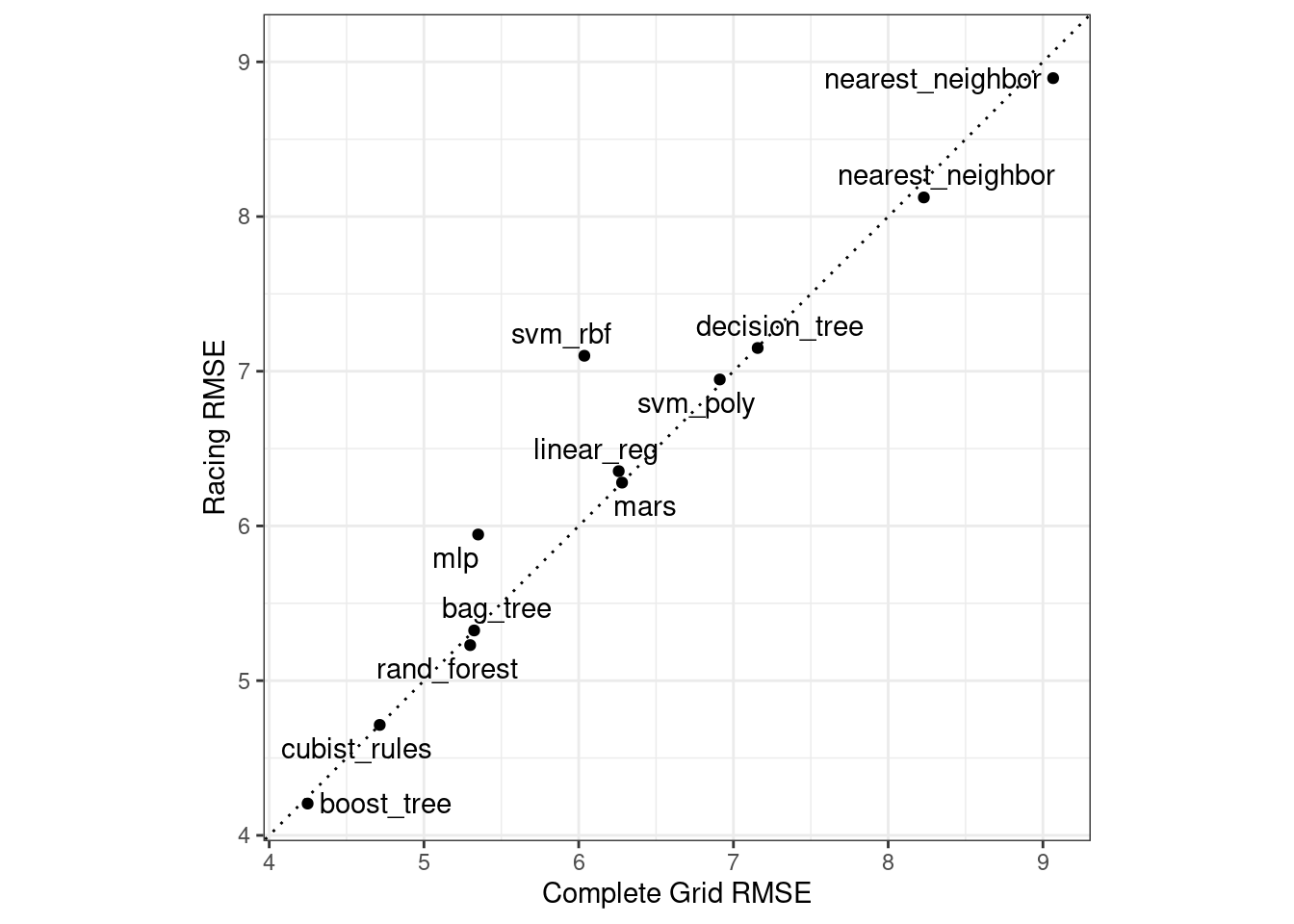
Figure 15.4: Estimated RMSE for the full grid and racing results.
While the racing approach selected the same candidate parameters as the complete grid for only 41.67% of the models, the performance metrics of the models selected by racing were nearly equal. The correlation of RMSE values was 0.968 and the rank correlation was 0.951. This indicates that, within a model, there were multiple tuning parameter combinations that had nearly identical results.
15.5 Finalizing a Model
Similar to what we have shown in previous chapters, the process of choosing the final model and fitting it on the training set is straightforward. The first step is to pick a workflow to finalize. Since the boosted tree model worked well, we’ll extract that from the set, update the parameters with the numerically best settings, and fit to the training set:
best_results <-
   race_results %>%
   extract_workflow_set_result("boosting") %>%
   select_best(metric = "rmse")
best_results
#> # A tibble: 1 × 7
#>   trees min_n tree_depth learn_rate loss_reduction sample_size .config
#>   <int> <int>      <int>      <dbl>          <dbl>       <dbl> <chr>
#> 1  1957     8          7     0.0756    0.000000145       0.679 Preprocessor1_Model04

boosting_test_results <-
   race_results %>%
   extract_workflow("boosting") %>%
   finalize_workflow(best_results) %>%
   last_fit(split = concrete_split)
We can see the test set metrics results, and visualize the predictions in Figure 15.5.
collect_metrics(boosting_test_results)
#> # A tibble: 2 × 4
#>   .metric .estimator .estimate .config
#>   <chr>   <chr>          <dbl> <chr>
#> 1 rmse    standard       3.41  Preprocessor1_Model1
#> 2 rsq     standard       0.954 Preprocessor1_Model1
boosting_test_results %>%
collect_predictions() %>%
ggplot(aes(x = compressive_strength, y = .pred)) +
geom_abline(color = "gray50", lty = 2) +
geom_point(alpha = 0.5) +
coord_obs_pred() +
labs(x = "observed", y = "predicted")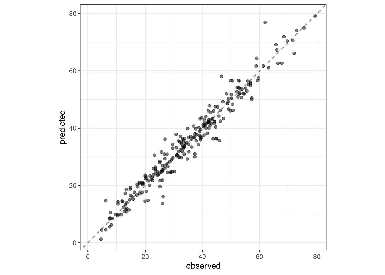
Figure 15.5: Observed versus predicted values for the test set.
We see here how well the observed and predicted compressive strength for these concrete mixtures align.
15.6 Chapter Summary
Often a data practitioner needs to consider a large number of possible modeling approaches for a task at hand, especially for new data sets and/or when there is little knowledge about what modeling strategy will work best. This chapter illustrated how to use workflow sets to investigate multiple models or feature engineering strategies in such a situation. Racing methods can more efficiently rank models than fitting every candidate model being considered.
REFERENCES
As of February 2022, we see slightly different performance metrics for the neural network when trained using macOS on ARM architecture (Apple M1 chip) compared to Intel architecture.↩︎